colours of my tea

a bit too strong!

I drink white and green tea black, but black tea white.

Isn’t language wonderful!

---

For all my social networking posts, see my Google+ page

computation limits physics

A self-replicating computer made of water (in theory).

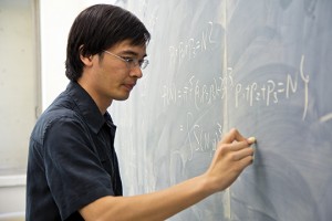
Terrence Tao tackles Navier-Stokes

---

For all my social networking posts, see my Google+ page

New Testament = Cinderella

Infographic of Kurt Vonnegut’s theory of the shapes of stories.

(via BoingBoing)

---

For all my social networking posts, see my Google+ page

sequestering carbon, several books at a time XIX

Hardly enough to be worth mentioning, but here is the latest lot:

problems, problems

John Baez lays out his approach to solving problems – interesting if you are spending your life at the task (ie, are an academic!)

---

For all my social networking posts, see my Google+ page

a surfeit of packaging

My phone started behaving strangely over the weekend: switching off for no reason, then claiming the battery was dead, but when I plugged it in to the charger, claiming the battery was half, then fully, charged.  After some searching on the web, I discovered this probably meant the battery was pining for the fjords.  Maybe not that surprising: it is 2 and a half years old, and has been maxed out on certain games at times.

More hunting on the web, and I found a place selling genuine Samsung batteries (as opposed to much cheaper batteries that the reviews seem to think are rip-offs) at eye-watering prices (I shouldn’t be surprised at the price, I suppose; I recently bought a new battery for my watch, and previously a new strap: the combined price was more than that of the original watch).  I ordered one; it arrived promptly today; the phone is now fine.  I have my life back.

Phone batteries are small and compact, so I was expecting a small parcel.  I received the battery in a plastic wrapper, in a jiffy bag, in a plastic envelope:

a lot to recycle…

the chaos game

By iteratively applying specific sets of transformations to the unit square, we can generate fractals.  For example, the famous Sierpinski triangle can be generated from three simple transformations:

Three transformations (shown in black, red, green), shown by their action on the unit square (grey), produce the Sierpinkski triangle

Rather than iteratively transforming shapes (the base Iterated Function System approach), these plots are produced using the “chaos game” algorithm: start with a random point, and plot its position as it is successively transformed by a random choice of transformation:

x := rnd
repeat
   choose transform w_i with probability p_i
   x := w_i(x)
   plot x

The resulting plot converges to the relevant fractal.

Different sets of transformations give different fractals.

Here, the black and green transformations are as before, but the red transformation includes a rotation

One nice feature of this approach is that smoothly changing the transformations smoothly changes the fractal.

Of course, there can be more than three transformations:

A pentagonal fractal produced by five transformations

The transformations don’t all have to have the same scale factors:

A “snowflake” produced from four transformations, one with a smaller "shrinkage" than the others

This is where the probabilities in the algorithm come into play.  When all the transformations have the same scale factor, we can choose transformations with a uniform random distribution.  When different scale factors are used together, a good heuristic is to choose transformations with probabilities weighted by the area of the relevant transformed square (given by the determinant of the transformation matrix).

The transformations don’t actually have to be squares: we can have different scalings in different directions, and shears, giving more complicated looking fractals:

A “coral tree”

And then we can smoothly transform between quite dissimilar fractals, by linear interpolation between their transformation sets:

From pentagon to coral, and back.

Probably the most famous fractal of this form is the “Barnsley fern”.

What is marvelous for playing about with these systems is that the plots can be produced with very little code: the code to define the transforms, plot the points, and construct the animated gifs, outweighs the core of the chaos game algorithm itself.

The Burden of the Bookish

Oh, how I recognise the thought processes involved here!

And Magic, Science and Religion and other essays by Bronislaw Malinowski, that could have some rich morsel ripe for the spinning in some fringe show or other, and if it is no use, I can always pass it on to Alan Moore. The Consolation of Philosophy by Boethius? I am sure I will get around to reading that, and if not, it matches all the other Penguin Classics I haven’t read that look nice in a row.

And fortunately (or maybe not?), I don’t have to worry what my other half will say about my habit – he’s as bad as me.

---

For all my social networking posts, see my Google+ page

so doge. much funny. wow

Why do shiba inus speak ungrammatically?  A linguist explains.

(via BoingBoing)

---

For all my social networking posts, see my Google+ page

windy!

There’s a saying: “there’s no such thing as bad weather, only bad clothes.”

I’m curious: what are the good clothes that would stop me from being blown over?

---

For all my social networking posts, see my Google+ page

book review: Inside Jokes

Matthew M. Hurley, Daniel C. Dennett, Reginald B. Adams, Jr.
Inside Jokes: using humor to reverse engineer the mind.
MIT Press. 2011

---

This started life as Hurley’s dissertation, but fear not: it is not some dull stodgy academic treatise. Despite being peppered with jokes, however, it is also not a side-splitting read. It is instead a clearly written in-depth account of the authors’ evolutionary cognitive theory of humour. The overarching argument is (roughly):

• All our behaviour, including thinking, is guided by emotions: without some emotional prod we would never make any actual decisions.
• Our emotions have evolved to produce rational behaviours (most of the time).
• Our thinking and decision-making usually needs to be done in real time: we need to react to the tiger now, not once we’ve finished evaluating all the possibilities.
• If we reason speedily with limited and uncertain information, we will make mistakes.
• These mistakes need to be fixed, to stop our mental space becoming clogged up with incorrect inferences.
• Correcting mistakes is hard work, so we have evolved an emotional "reward": mirth, which we experience when we consciously recognise an unconsciously committed incorrect belief (modulo some further conditions).
• This emotion, like others, can be exploited to new ends: here, humour and comedy.

This thesis is introduced in the context of an emotional and cognitive model of how we think. Emotion is clearly important in things like “fight or flight”, but also for many other aspects of our life. Certain forms of brain damage that inhibit emotions make it difficult or impossible for those people to make decisions: not because they can no longer reason, but because they have no urge to make a decision. Thinking itself is such hard work, we need emotions to encourage us to do so.

p79. Boredom has its place in driving us out from cognitive malaise. Though curiosity inspires our cognitive apparatus into detailed exertion surrounding particular as-of-yet-unexplained regularities, we would scarcely commence toil at all without the dull pain of boredom to keep us from the simple irresponsibility of just doing nothing. If there is no pressing topic to think about, we still think, and incessantly so, because it hurts not to.

Although we think incessantly, at times we need to think quickly, and to make a decision before we have all the information. There is an evolutionary advantage to literally jumping to conclusions: those that pondered more deeply were eaten. But if we don’t have all the information, inevitably we will make mistakes, no matter how well evolution has honed our conclusion-jumping heuristics into rational emotional behaviours.

p82. Choosing how to behave under uncertainty requires a heuristic choice process. Good heuristics give excellent approximations much of the time. But, in the (restricted-by-design) areas where they fail, they give predictably—even pathologically—poor results. The emotions are rational, but the system is a heuristic driver of behavior that operates on incomplete information; so we must accept that the emotions will fail us in some ways, such as overreactions and addictions, that are irresolvable.

Mistakes can be dangerous, as they will include false information about the world, which later will pollute the very reasoning we need in order to survive. So we have evolved mechanisms to help us correct these mistakes.

p120. The need, then, is for a timely and reliable system to protect us from the risks entailed by our own cleverness. Discerning and locating these mistakes would have the immediate payoff of allowing current reasoning to progress without an error (before we act on such errors), but would also provide a legacy for the future, keeping a fallacious conclusion from becoming registered as verity in long-term memory. A mechanism for consistency checking is indispensable for a system that depends crucially on data-intensive knowledge structures that are built by processes that have been designed to take chances under time pressure. Undersupervised and of variable reliability, their contributions need to be subjected to frequent “reality checks” if the organism that relies on them is to maintain its sanity.

However, this error correction is expensive, and is competing for the same resources that the original thought uses. Something expensive needs some reason to happen. This is the key to the authors’ model: the reason is the evolved reward mechanism of mirth. Sweet foods are not intrinsically “sweet”; we experience them as sweet (a pleasant emotional response) because we are evolved to find them so: sugar was a rare and valuable energy source. Similarly, jokes are not intrinsically “funny”; we experience them as funny (a pleasant emotional response) because we are evolved to find them so: error correction is a valuable cognitive function.

Having introduced their thesis, the authors then subject it to various challenges. It needs to account for the diverse range of things we find funny, and yet should also explain why closely related things are not funny. They do this in considerable detail, picking apart and analysing a wide range of humorous and related event. Of course, picking apart a joke destroys its humour; interestingly, the theory even explains why it destroys the humour.

This is a fascinating and well-argued account of a particular aspect of our evolutionary heritage. Recommended. (Some of the example jokes included are even funny.)

---

For all my book reviews, see my main website.

sequestering carbon, several books at a time XVIII

A new batch, accumulated over the last couple of weeks:

arms, legs, and...?

I’ve been looking up norovirus symptoms. (Yes, thank you, it is unpleasant.)  I found the statement:

Norovirus originates in the gastrointestinal system and often causes aching limbs, especially the arms and legs.

Interesting: how many other limbs are there?

this person is only acting ill

---

For all my social networking posts, see my Google+ page

finding Brazil

While scanning the BBC news on my phone, I noticed an item about Brazil, where the thumbnail image was a map of Brazil.  To help identify where Brazil is, just in case you don’t know, there was an inset map.  I’m not sure it provides that much extra help.

---

For all my social networking posts, see my Google+ page

writhing spots

We’ve been watching the massive sunspot currently visible on the sun with fascination.

Phil Plait talks about it, and provides a marvelous video, showing the dynamism of the “spots“: how they writhe and move.

---

For all my social networking posts, see my Google+ page

solar stats for January

I blogged the detailed solar power generation through the day for the first few days after we had the system installed.  Not we have more data, here are the plots for all of January (starting on the 9th), using Tuftian "small multiples".

Data is gathered at 10 minute intervals. The horizontal time axis runs from 3:00am to 9:00pm GMT. The vertical axis runs from zero to 8kW. The orange regions indicate the lower quartile, median, upper quartile, and maximum generation at that time, over the month. (Click to embiggen.)

That shows very well how variable the weather can be, from day to day, and from hour to hour.

Each day’s generation can be integrated, to show total power per day.

Daily power generation, in kWh (grey bars), along with a running average (lower quartile, median, upper quartile, maximum; orange areas), over the previous 7 day sliding window.

And that also shows how variable the weather can be from day to day, and how January got steadily gloomier.  But even a median generation of 10kWh/day is better than a poke in the eye with a burnt stick.

Rather than continually blog about all this, I’ve set up a page on my other website, which will keep the up-to-date charts.

quantum walking

It’s possible to build a quantum random walk simulator in Python/NumPy with code that is very close to the mathematical definitions.  Here’s how.

First, we need to import NumPy (to do the array operations) and matplotlib (to visualise the results).

from numpy import *
from matplotlib.pyplot import *

We define the number of steps, +++N+++, that we are going to walk.  We also define the total number of different positions the walker can be in after +++N+++ steps.

N = 100      # number of random steps
P = 2*N+1    # number of positions

a quantum coin

We toss a quantum coin to decide whether to go left or right (or a superposition).  In ket notation, we can write a general quantum coin as an arbitrary superposition of two states:
$$| coin \rangle = a | 0 \rangle_c + b | 1 \rangle_c; \mbox{ where} |a|^2 + |b|^2 = 1$$
The ket notation is a convenient shorthand for the actual vectors representing the state:
$$| 0 \rangle_c  = \left( \begin{array}{c}
1  \\
0  \end{array} \right);\ | 1 \rangle_c  = \left( \begin{array}{c}
0  \\
1  \end{array} \right)$$
So we can use a NumPy array to define a coin state:

coin0 = array([1, 0])  # |0>
coin1 = array([0, 1])  # |1>

the Hademard coin operator

We will see terms like +++| 0 \rangle_c \langle 0 |+++ in what follows.  This is the outer product of the relevant vectors, resulting in a matrix.  We can use NumPy to calculate these:

C00 = outer(coin0, coin0)  # |0><0| 
C01 = outer(coin0, coin1)  # |0><1| 
C10 = outer(coin1, coin0)  # |1><0| 
C11 = outer(coin1, coin1)  # |1><1| 

Quantum operators are unitary matrices.  The coin operator, that can be used to flip a quantum coin into a superposition, is:
$$\hat{C} = \frac{1}{\sqrt{2}} \left( | 0 \rangle_c \langle 0 | + | 0 \rangle_c \langle 1 | + | 1 \rangle_c \langle 0 | - | 1 \rangle_c \langle 1 | \right)$$

C_hat = (C00 + C01 + C10 - C11)/sqrt(2.)

position on a line

In ket notation, we can write the fully general position of the walker on the line as an arbitrary superposition of the +++P+++ possible states:
$$| posn \rangle = \sum_k \alpha_k | k \rangle_p ; \mbox{ where} \sum_k | \alpha_k |^2 = 1 $$

shift (step) operator

The step operator moves left or right along the line, depending on the value of the coin:
$$\hat{S} = | 0 \rangle_c \langle 0 | \otimes \sum_k | k+1 \rangle_p \langle k | + | 1 \rangle_c \langle 1 | \otimes \sum_k | k-1 \rangle_p \langle k |  $$
We assume the line is actually on a circle, so the positions at the ends wrap around.  However, we will always make the circle big enough so that this doesn’t happen during a walk.  The tensor product +++\otimes+++ is implemented with the NumPy kron operation:

ShiftPlus = roll(eye(P), 1, axis=0)
ShiftMinus = roll(eye(P), -1, axis=0)
S_hat = kron(ShiftPlus, C00) + kron(ShiftMinus, C11)

walk operator

The walk operator combines the coin operator on the coin state, and a step operator on the combined coin and position state:
$$\hat{U} = \hat{S} \left( \hat{C} \otimes \hat{\bf I}_p \right)$$

U = S_hat.dot(kron(eye(P), C_hat))

initial state

Let’s take the initial state of the system to be a coin in a superposition of left and right, and the walker at position 0:
$$ | \psi \rangle_0 = | coin \rangle_0 \otimes | posn \rangle_0 = \frac{1}{\sqrt{2}} \left( | 0 \rangle_c + i | 1 \rangle_c\right) \otimes | 0 \rangle_p$$

posn0 = zeros(P)
posn0[N] = 1     # array indexing starts from 0, so index N is the central posn
psi0 = kron(posn0,(coin0+coin1*1j)/sqrt(2.))

state after +++N+++ steps

Then walking +++N+++ steps is just applying the walk operator +++N+++ times:
$$ | \psi \rangle_N = \hat{U}^N | \psi \rangle_0$$

psiN = linalg.matrix_power(U, N).dot(psi0)

And we’re done! +++ | \psi \rangle_N+++ is the state of the system after +++N+++ random quantum steps.

measurement operator

We can measure the state at position +++k+++ using the measurement operator
$$\hat{M}_k = \hat{\bf I}_c \otimes | k \rangle_p \langle k |$$
We can use this to build up an array of probabilities, by taking the modulus squared of the state value at each position. (We can calculate the whole distribution in one go in simulation, but we would only get one measurement per experiment on the real quantum system.)

prob = empty(P)
for k in range(P):
    posn = zeros(P)
    posn[k] = 1     
    M_hat_k = kron( outer(posn,posn), eye(2))
    proj = M_hat_k.dot(psiN)
    prob[k] = proj.dot(proj.conjugate()).real

plot the distribution

We can then plot the probabilities.

fig = figure()
ax = fig.add_subplot(111)

plot(arange(P), prob)
plot(arange(P), prob, 'o')
loc = range (0, P, P / 10) #Location of ticks
xticks(loc)
xlim(0, P)
ax.set_xticklabels(range (-N, N+1, P / 10))

show()

For +++N=100+++ we get

probability distribution for a quantum random walk with +++N=100+++, symmetric initial coin

The maximum probability occurs at +++\approx N/\sqrt{2}+++.

If instead of starting with a symmetric initial coin, we start with +++|0\rangle_c+++, we get

probability distribution for a quantum random walk with +++N=100+++, initial coin +++|0\rangle+++

In neither case do these look anything like the bell curve of a classical random walk, with its maximum probability at +++0+++.  If you are drunk and trying to stagger home, best be quantum!

What I find most impressive about the Python is how closely we can make the code follow the mathematical formalism thoughout.