Showing posts with label algorithm. Show all posts

Saturday, 20 June 2026

stacking up

I thought yesterday's SeeStar shot of the moon was good.

But my other half also took a SeeStar video of it.  Why would you take a video of a static scene?  To enhance the view.  He spent today fiddling around with AutoStakkert!, software to stack multiple frames to get a better image.  The result is great, much crisper:


Why not just use the SeeStar to integrate over a longer time, like with other images?  Well, it doesn't do that for solar system objects, so we just have to try harder.

He also played around with a solar video taken at the end of May.  Here's a simple image:

2026/05/29, 17:48 BST

And here's the result of processing the video, with much more detail visible on the sunspots:


Monday, 26 January 2026

sequestering carbon, several books at a time CLVII

The latest batch, including a few belated Christmas presents that were ordered well in advance, but delivered less so.


Tuesday, 7 October 2025

ALife 2025 day 2

Tuesday, and the full conference gets going.  

We started with a great keynote from Hector Zenil, on using Kolmogorov Complexity measures.  Just because it is uncomputable doesn't mean it is useless.  Most of mathematics is undecidable, but that doesn't stop us using maths!  We shouldn't just give up and use simple lossless compression algorithms. We can do better, and getter better bounds, better approximations, by trying harder and harder (running the search algorithm for longer), which means we can be better at filtering out randomness from things that superficially look random, but that have algorithmic patterns.  It was a fascinating talk.  I've had Hector's book on Algorithmic Information Dynamics on my to-read pile for a while now -- I need to bump it up nearer to the top.

Then on to the contributed papers.  During one of these, on Synthetic Ecosystems, I became one of today's "Lucky 10,000", when I discovered that until relatively recently, Ascension Island was an essentially lifeless desert.  Darwin stopped there on his way home, and decided it needed "greening".  Today, after a lot of work, it has a lush, totally artificial, ecosystem!

The poster session has lots of interesting work on display, including a contribution by my student.  There were also some beautiful "Analogue Atomic Automata": large, carefully grown bismuth crystals, by Solvi Arnold:


In the evening we had a fascinating online keynote from Michael Levin, on biological embodiment, agential material, and bioengineering.  It might have been 8pm for us, but it was 7am for him!  (We live on a sphere.)


Monday, 6 January 2025

Raman SOM

Daniel West, Susan Stepney, Y. Hancock.  Unsupervised self-organising map classification of Raman spectra from prostate cell lines uncovers substratified prostate cancer disease states.  Scientific Reports, 15:773, 2025. doi:10.1038/s41598-024-83708-6

This started out as a feasibility study, to see if Kohonen Self-Organising Maps (SOMs) could be used to cluster minimally preprocessed Raman spectroscopy data taken from individual cells.  SOM an unsupervised learning approach, and can cluster high dimensional data (here, over 1000D) down into a 2D visual representation.  We had Raman spectra of prostate cells, some cancerous, some not.  Could a SOM distinguish these two classes?

We blinded the data, so that the system did not know which spectrum was in which class, to ensure this was truly an unsupervised exercise.  After some fiddling about to understand what values several parameters should be, we fed the data in, and looked at the resulting map.  We could see three clusters.

Had it worked?  We unblinded the data, and yes, one of the clusters was the non-cancerous cells, and the other two clusters were cancerous cells.  Why two clusters?  Well, it turns out the mapping process had managed to discover two distinct classes of cancerous cells.  Further research is underway to investigate these differences.

So yes, it works, and better than we had hoped!


Monday, 13 March 2023

UCNC day 1

It's the first day of Unconventional Computation and Natural Computation 2023 conference.

It started off with a great keynote by Thomas Bäck, titled "On the automatic optimisation of problem-specific optimisation heuristics gleaned from nature".  Many population-based optimisation algorithms are essentially variations on a theme, with different parameter settings.  Rather than invent yet another variant, instead, optimise the parameter settings for your particular application.  This can lead to "weird" algorithm configurations, but better ones than we can design by hand.  Then, what to do if your cost function is too expensive to calculate for this approach? Then use a suitable cheaper proxy for the tuning, and use the tuned algorithm on the real problem.  However, standard benchmarks aren't good proxies, so use a random function generator, and choose results that are good proxies.  (And there was more good stuff too, but noting it here would make this post too long: go read his papers instead!)

Next was supposed to be the first half of the TEMC (Theoretical and Experimental Material Computing) workshop that I was running.  Unfortunately, my invited speaker was not having the same smooth travel experience from Canada that I had experienced from the UK, and wasn't going to arrive until lunchtime.  So I liaised with the conference organiser to swap some talks around.  

So instead, we had a session of conference presentations by my team, on quantum computing and reservoir computing.

After lunch, Ion Petrie delivered an invited tutorial on Reaction Systems.  I had come across these before, but it was good to have a session putting everything in one place.

Last but not least, my workshop speaker, Julien Sylvestre, gave a fascinating invited talk on unconventional robotics: using unconventional computational models in concert with unconventional hardware.

So, a great opening to the conference.  Off to the evening welcome reception at a beach-front venue.


Monday, 5 July 2021

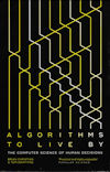
book review: Algorithms to Live By

Brian Christian, Tom Griffiths.
Algorithms to Live By: the computer science of human decisions.
Collins. 2016
This book does several things very well indeed. It introduced a broad range of Computer Science’s fundamental algorithms, explaining them simply and clearly. It shows how we might apply these algorithms in our everyday lives, to help us make more efficient and effective decisions. And it shows that even when we have the provably best means of making a decision, it might not always (or even very often) work.

It covers approaches to searching, and when to stop looking for improvements over what you already have. It discuses sorting, and tradeoffs between time spent keeping things in order, and time spent finding them later. It covers scheduling, and how the best order to do things in depends very much on what you are trying to optimise. It finishes with game theory, explaining why some situations lead to poor outcomes for all, and how understanding this can help you know how to change the situation to get better outcomes. And it does all this, and more, with a light touch that makes it very readable.


For all my book reviews, see my main website.

Saturday, 27 October 2018

sequestering carbon, several books at a time XC

The latest batch, including a few venerable old titles purchased from a retiring colleague.


Thursday, 25 October 2018

using domain knowledge to evolve graphs

We are investigating using evolutionary algorithms to evolve graph structures directly, and are getting some rather nice results.

One thing that’s made a lot easier by using an explicit graph representation is encoding domain knowledge about “semantics preserving mutations”.  This allows domain specific neutral mutations to be added easily.  Since neutral mutations are supposed to help evolution, this should be good?  And yes, it is!

Our latest paper, just up on the arXiv, shows how including certain propositional logic tautologies, such as de Morgan’s laws, as neutral mutations, makes for imporved performance when evolving benchmark circuits.

Timothy Atkinson, Detlef Plump, Susan Stepney
Semantic Neutral Drift
arXiv:1810.10453 [cs.NE]

We introduce the concept of Semantic Neutral Drift (SND) for evolutionary algorithms, where we exploit equivalence laws to design semantics preserving mutations guaranteed to preserve individuals’ fitness scores. A number of digital circuit benchmark problems have been implemented with rule-based graph programs and empirically evaluated, demonstrating quantitative improvements in evolutionary performance. Analysis reveals that the benefits of the designed SND reside in more complex processes than simple growth of individuals, and that there are circumstances where it is beneficial to choose otherwise detrimental parameters for an evolutionary algorithm if that facilitates the inclusion of SND.


Saturday, 6 January 2018

Amazon search fail ... or is it?

Rather aggressive and incorrect auto-correct by Amazon’s search bar:


Despite it searching not for what was asked for, but for what it thought was asked for, it nevertheless found what was asked for.  So only semi-fail.

Interestingly, searching just for “judith merril” does not result in “merril” being changed to “merrell”.

Computers.  Doncha just love ’em?


Saturday, 14 October 2017

multi-objective optimisation II

In a previous post, I described what a Pareto front is, and Deb et al (2000)’s algorithm for finding it.  We have the first element we need for a multi-objective optimisation algorithm.  There is one more subtlety first, though.

We want to get a good estimate of the whole Pareto front, not just a few points on it.  So we want the points we find to be well spread out across the front.  Deb et al define the crowding distance: we prefer less crowded to more crowded points, as the densely crowded ones are not giving us much extra information about the front.  Their algorithm is:


Here, I is the set of points, and I[i].m is the value of the mth objective function of the ith individual in I.  We can code this up in python as follows (with I being a list of points in a particular front):
def crowding_distance_assignment_single_front(pfront):
  # pfront = list of individuals, dictionary { 'state':s, 'fitness':(f1, ... fm) }
  inf = 1000000                  # "infinity"
  dist = [0] * len(pfront)       # list of distances, I_distance
  m = len(pfront[0]['fitness'])  # no of objectives (= size of 'fitness' tuple)
  for mi in range(m):
    # sifront = [(i, pfront[i]), ...] sorted on mi-th fitness values of pfront
    # sifront[j][0] = original index i of item in pfront list
    # sifront[j][1]['fitness'][mi] = mi-th fitness value of jth sorted individual
    sifront = sorted(enumerate(pfront), key=lambda x:x[1]['fitness'][mi]) 
 
    dist[sifront[0][0]] += inf    # first boundary item in list
    dist[sifront[-1][0]] += inf   # last boundary item in list
    for i in range(1,len(sifront)-1):       
      dist[sifront[i][0]] += sifront[i+1][1]['fitness'][mi] \
                             - sifront[i-1][1]['fitness'][mi]

  # sort pfront into reverse distance order, using distance list
  dist, pfront = (list(t) for t in 
                  zip(*sorted(zip(dist,pfront), key=lambda x:x[0], reverse=True)))

  return(pfront)
The algorithm works by sorting the list of individuals in order of their fitness value for objective mi.  The distance value of each point is the sum of the distances to its two neighbouring points: crowded points will have low distances, so low distances are bad.  The first and last points in the list are given a very high (good) value.  This is repeated for each objective dimension, adding up the distance measures.

The python then does one more thing than the Deb et al algorithm.  It uses the distances calculated to sort the original list of individuals into reverse distance order (high distance isolated points near the the front, low distance crowded points towards the end) and returns that sorted list.

Then we can sort the list of fronts in the obvious way:
def crowding_distance_assignment(pfrontlist):
  for i, pfront in enumerate(pfrontlist):
    pfrontlist[i] = crowding_distance_assignment_single_front(pfront)
  return(pfrontlist)
Now we have enough to make a multi-objective search algorithm:
Np = 100        # parent population size
Nq = 100        # no of children
Ngen = 250      # no of generations
Nstate = 3      # size of individual state

parents = init_popl(Np,Nstate)
children = make_children(parents, Nq)

for _ in range(Ngen):
    popl = parents + children
    # construct the list of fronts from the population (previous post) 
    pfrontlist = fast_nondominated_sort(popl)              
    # sort each front into least crowded (highest distance) order
    pfrontlist = crowding_distance_assignment(pfrontlist) 

    # new parents become the best of the previous popl of parents + children
    parents = [item for pfront in pfrontlist for item in pfront][:Np]  
    # make new children from those parents 
    #  note that parents are sorted in fitness order    
    children = make_children(parents, Nq)                                    
We need to define init_popl() to build some initial (usually random) population.
import random
def init_popl(n,nstate):
    # return list of n individuals, each with nstate state vars, each in -1..1    
    pop = []
    for _ in range(n):                      
      state = tuple([random.uniform(-1,1.) for i in range(nstate)])
      pop += [{'state': state, 'fitness': fitness(state)}]        
    return pop
Here I have simply hardcoded in an initial range of +/-1, because I am demonstrating this with the equally hard-coded Kursawe function objectives:
import math
def fitness(state):
    # Kursawe function
    x1,x2 = state
    f1 = -10*math.exp(-0.2*math.sqrt(x1**2+x2**2)) \
        - 10*math.exp(-0.2*math.sqrt(x2**2+x3**2))
    f2 = abs(x1)**0.8+5.*math.sin(x1**3) \
       + abs(x2)**0.8+5.*math.sin(x2**3) \
       + abs(x3)**0.8+5.*math.sin(x3**3)
    return(f1,f2)
Now all that’s left is to define make_children(), which breeds the next generation. Deb et al simply say “Binary tournament selection, recombination, and mutation operators are used to create a child population”.  So, for the sake of demonstration, let’s do the simplest possible thing here: binary tournament with a fixed mutation of the three component state, and no recombination:
def make_children(parents, nq):
    # parents = list of items in fitness order, fittest first 
    #   (except on v first call)
    # nq = no of children to make
    
    # tournament selection + mutation
    np = len(parents)
    children = []
    for _ in range(nq):
        # binary tournament: chose two parents randomly
        p12 = random.sample(range(np),2)
        # tournament winner = lower number, because sorted
        p = parents[min(p12)]  
        s = mutate(p['state'])
        children += [ {'state': s, 'fitness': fitness(s)} ]
    return children

def mutate(state):
    x,y,z = state
    return (x+random.uniform(-0.1,0.1), 
            y+random.uniform(-0.1,0.1), 
            z+random.uniform(-0.1,0.1)) 
Clearly, init_popl(), fitness(), make_children(), and mutate() should be modified into general purpose code, but that’s not the point of this post.

Here are some results, for the Kursawe function, and for a population size of 100 (click to get a larger view).
After 2 generations: (top left) fitness/objective values (f1,f2), with the current fronts of the entire population as calculated using fast_nondominated_sort(), and different front plotted in different colours; (top right) the corresponding (x1,x2) state space (x3 omitted for clarity) of the entire population, with the points plotted in the same colours as in the fitness plot; (bottom left) the fittest front only, plotted with a rainbow colouring along its length; (bottom right) the state space corresponding to the fittest front, with the points plotted in the same colours as along the front.
After 25 generations; plots as above.  The fronts are converging, and the Pareto front is becoming clear.  The states corresponding to different positions on the Pareto front (that is, to different tradeoffs between the objectives) are also becoming clear. 
After 250 generations.  The Pareto front is fully defined and evenly filled; the corresponding state values are well clustered.
After 250 generations with no call of the crowding_distance_assignment() function.  The Pareto front is less well defined, and less evenly populated.
So that’s it!  Deb et al’s multi-objective optimisation algorithm, in python.

Reference

Deb, Kalyanmoy; Agrawal, Samir; Pratap, Amrit; Meyarivan, T. (2000) A Fast Elitist Non-dominated Sorting Genetic Algorithm for Multi-objective Optimization: NSGA-II. In Parallel Problem Solving from Nature, PPSN VI. LNCS 1917:849–858. Springer. doi:10.1007/3-540-45356-3_83

Wednesday, 11 October 2017

multi-objective optimisation I

There are lots of optimisation algorithms around: I’ve used simulated annealing and evolutionary algorithms, to name but two.  However, I’ve only ever used them to optimise a single value.  But real problems often have multiple objectives to satisfy simultaneously: time, price, and quality is a traditional triple.  However, multiple objectives are often in conflict, and so it is not possible to optimise them all simultaneously: there are tradeoffs.  “Pick any two of three” is the stated tradeoff for time, price, and quality; more nuanced tradeoffs are available.

One common technique is simply to add the various objective values together, with some weight for each, to reduce the problem to a single optimisation.  But which weights?  Different weights imply different tradeoffs.

So the next step is a full multi-objective optimisation system.  To see what is going on, the crucial concept of dominated solution needs to be understood.

Let’s assume that a candidate solution s has objective values (f1, f2, ..., fn).  And let’s assume we want to minimise each of those objectives (the maximisation case is similar, mutatis mutandis).  Then solution s1 dominates solution s2 if every one of its objective values is less than the corresponding value for s2.  If on the other hand, s2 is better in all its objectives than s1, then s2 dominates s1.  And in the case when neither dominates the other, these solutions are non-dominated.  The figure below illustrates these concepts.

Candidate solutions plotted in some in 2D objective space, where we wish to minimise both objectives.  Consider the central red solution.  It dominates all candidate solutions in the upper right quadrant, because both its objective values are better than those in the dominated quadrant.  It is dominated by all candidate solutions in the lower left quadrant, because both its objective values are worse than those in that quadrant.  The other two quadrants are non-dominated solutions: one objective is better, but the other is worse.  The large green dots along the lower edge represent solutions on the Pareto front: all the solutions that are not dominated by any other candidate.  The concepts generalise to higher dimensions when there are more than two objectives.  
We can write a simple python function to calculate whether one solution dominates another, for an arbitrary number of objectives:
def dominates_min(a,b):   # for minimisation problems
  # a and b are nD tuples of the respective n objective values
  # a dominates b if a.x < b.x and a.y < b.y and ...
  return all([(a < b) for a, b in zip(a,b)])
How this works:  Let the tuples by (ax, ay, az) and (bx, by, bz).  Then zipping them together gives the list of tuples [(ax,bx),(ay,by),(az,bz)].  The set comprehension gives a list of booleans, True or False depending if the respective ai<bi or not.  Then the all function tests whether all the values are True.
In a complete collection of candidate solutions, the ones not dominated by any other solution form the Pareto front.  These are the best possible solutions: no other candidate performs better in all objectives.  The front describes the possible tradeoffs: values along the front represent different tradeoffs.

When we don’t have all candidate solutions to hand, maybe just a sample of solutions, we need an optimisation algorithm to find those candidates close to the actual Pareto front, and to use them to find even better ones.

But first, we need to calculate the points on the Pareto front of a given population, that is, all the candidate solutions that are not dominated by any other solutions (the green points in the figure above).  The obvious algorithm (for each candidate solution, test it against all other solutions for all objectives) is rather inefficient, being O(MN2), where M is the number of objectives, and N is the number of solutions to test.  Deb et al (2000) give a more efficient algorithm:


We can code this up in python as follows (with comments showing how it relates to the algorithm above):
def fast_nondominated_sort_single_front(pop):
  # pop = list of individuals
  #   individual of form { 'state': (s1,s2,s3,...), 'fitness':(f1,f2,f3,...) }
  # pfront = list of individuals on the calculated "pareto front"

  pfront = [ pop[0] ]      # P' = {1}
  for pi,p in enumerate(pop):  # for each p in P and p notin P'
    if pi == 0 : continue      # (so not the first element)

    pfront = pfront + [ p ]    # P' = P' cup {p}
    # make a copy to iterate over, because pfront is being modified; 
    #   don't need the last item, which is p  (makes q neq p below True)
    pfrontcopy = pfront[:-1]   

    pf = p['fitness']
    for qi,q in enumerate(pfrontcopy):    # for each q in P' and q neq p 
      qf = q['fitness']
      if dominates_min(pf,qf):     # if p dom q
        pfront.remove(q)           #   then P' = P' \ {q}
      elif dominates_min(qf,pf):   # else if q dom p
        del pfront[-1]             #   then P' = P' \ {p}
        break    # don't have to check any more qs as p already gone

  return(pfront)
Once we have the front, we could remove it from the population, and calculate the next front, and so on.  This is useful in an optimisation algorithm, to find less fit (not on the current best front) but still possibly good solutions, for use in building even better ones.

The multiple front calculation is as follows:
def fast_nondominated_sort(pop):
  # find a list of ever decreasing fronts
  # pop = list of individuals
  # pfrontlist = list of fronts = list of lists of individuals

  popcopy = pop[:]
  pfrontlist = []
  while popcopy:
    pfront = fast_nondominated_sort_single_front(popcopy)
    pfrontlist += [pfront]
    # remove the found pfront from the pop
    popcopy = [ ind for ind in popcopy if ind not in pfront ]  

  # check that no-one has been lost
  assert len(pop) == len([item for pfront in pfrontlist for item in pfront]) 

  return(pfrontlist)
Given some population of candidate solutions, we can plot out the relevant fronts so calculated (plotting code always seems much more complicated than the actual algorithms!):
import matplotlib.pyplot as plt
def plot_fronts(pfrontlist):
  # pfrontlist = list of fronts; each front is a list of individuals

  fig = plt.figure() 
  ax1 = fig.add_subplot(111) 

  # one colour per front 
  colors = matplotlib.cm.rainbow(np.linspace(0, 1, len(pfrontlist))) 
  # iterate backwards, to draw better fronts on top of less good ones 
  for i in range(len(pfrontlist)-1, -1, -1) :  
    pfront = pfrontlist[i]

    # sort members of front in order of fitness; draw a line along the front
    data = sorted([ pf['fitness'] for pf in pfront ]) 
    xs = [ i[0] for i in data ]
    ys = [ i[1] for i in data ]
    ax11.plot(xs, ys, ':o', color=colors[i], mew=0)
  plt.show()
This gives a plot like:
A sequence of fronts, found by finding the Pareto front of a population of candidate solutions, removing it from the population, finding the front of the remaining candidates, and so on.


In a later post, I will go through the rest of the Deb et al (2000) algorithm, and show how they incorporate this front-finding into a full-blown multi-objective optimiser.

Reference

Deb, Kalyanmoy; Agrawal, Samir; Pratap, Amrit; Meyarivan, T. (2000) A Fast Elitist Non-dominated Sorting Genetic Algorithm for Multi-objective Optimization: NSGA-II. In Parallel Problem Solving from Nature, PPSN VI. LNCS 1917:849–858. Springer. doi:10.1007/3-540-45356-3_83

Sunday, 30 July 2017

Tupper's self-referential formula

This video introduces Tupper’s self-referential formula.  The formula is both more, and less, amazing that it initially seems.


For all my social networking posts, see my Google+ page

Monday, 13 March 2017

visualising complex continued fractions

Thomas Baruchel's beautiful plots of complex continued fractions.


[via John Baez]

For all my social networking posts, see my Google+ page

Sunday, 29 January 2017

“I just showed that the bomb was there.”

Nerds enabling fascism?
Trump Knows You Better Than You Know Yourself 
with a mere ten “likes” as input his model could appraise a person’s character better than an average coworker. With seventy, it could “know” a subject better than a friend; with 150 likes, better than their parents. With 300 likes, Kosinski’s model could predict a subject’s answers better than their partner. With even more likes it could exceed what a person thinks they know about themselves. 
The world has been turned upside down. The Brits are leaving the EU; Trump rules America. And in Stanford the Polish researcher Michal Kosinski, who indeed tried to warn of the danger of using psychological targeting in a political setting, is still getting accusatory emails. “No,” says Kosinski quietly, shaking his head, “this is not my fault. I did not build the bomb. I just showed that it was there.”


For all my social networking posts, see my Google+ page