memories of snowbirds

Two weeks ago, the weekend that my machine died, there was the last of the snow (I hope). Snow seems to make birds more visible.  So we were watching the bird feeder through the window, and saw several new kinds of birds.  First there was this:

possibly a reed bunting

On consulting our trusty bird book, we decided it was a reed bunting (or possibly a mutant sparrow).  While we were trying to identify it, we noticed another little brown bird hopping around on the ground.  I confidently identified it as a distant sparrow, then looked through the binoculars, saw it had quite a streaked breast, and a thin beak, and swiftly lost my confidence.  After consulting the bird book again, we tentatively decided on meadow pipit (or very mutant sparrow).  Then it flew up into the apple tree: maybe it was a tree pipit?  The bird book helpfully points out distinguishing features in its diagrams, such as differences in colour on tails or wings; unfortunately, there are no features indicated to distinguish between meadow pipits and tree pipits. The text says that the tree pipit is distinguished "from meadow pipit by voice, habitat; also by buffer, less olivaceous colour, pinker legs", and that the meadow pipit "perches less frequently than the tree pipit"; not very helpful features if you have only the one specimen! (The same book helpfully dubs warblers "confusing". Yet despite all this, or maybe because of it, it is my bird identification book of choice.)

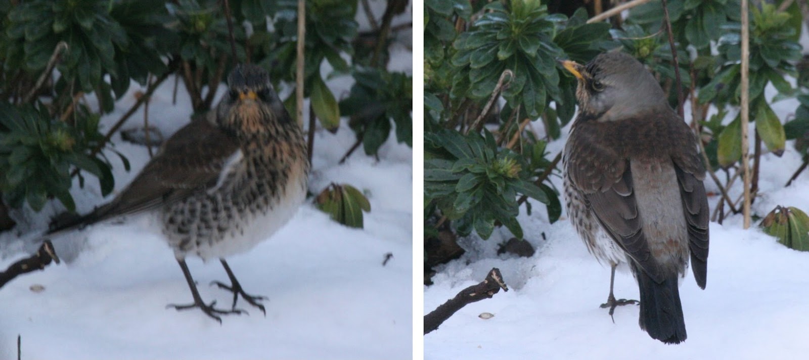
While we were debating these identifications, we noticed a larger, more brightly-coloured bird. positively glowing in the sunshine, perched on the large trunk of the apple tree.  What an earth is that?  Feverish page-turning.  No doubt about it this time, it was a fieldfare.  Not only had we never seen one before, I can safely say I'd never even heard of them before.  It flew down to the ground, and pirouetted for our benefit.

fieldfare, showing off for the camera (front shot a little out of focus)

Gorgeous.  Almost makes the snow worthwhile.

fieldfare behind the dogwoods

carry on installing

So, after the sad demise of my home PC last week, it is off to our local computer shop, World of Computers (an excellent place where we have been buying our machines for the last two decades at least), for its replacement.

Back home, I plug in all the peripherals, and now I have a beefy spookily quiet machine with all my data transferred on to it (so at least I don't have to restore from backup), but essentially no software.  This is Windows 7; given some of the software running on my previous XP machine had been ported to it eight years ago from my previous Win95 machine, I may be in for a hard time.

First things first -- I install the security software.

Then I download Chrome and Evernote, and I'm ready to start serious installation, including taking notes to help me next time.  I set the wallpaper to a Hubble Deep Field image, and I'm starting to feel at home again.

The first thing I notice is that there's a thick black border around my monitor screen, and the text is slightly fuzzy.  I remember this happening when I first got it, and that I did something that wasn't to do with setting the resolution; but beyond that -- no recall.  However, the web comes to the rescue:  googling the problem reminds me it is called "overscan/underscan" -- googling that tells me to use Catalyst Control Centre.  Which is not installed, so that's my next download.

Full screen de-fuzzified, I next install MS Office.  That's a 1GB download, leading me to wish, not for the first time, that our internet broadband was fibre, rather than some species of wet string.  The Office download page provides me with download instructions in a pdf.  So I download Adobe Acrobat Reader.  Then I look at the download instructions, which are all out of date.  But the download and installation proceeds normally without their help.

Then it's Texnic Center and MiKTeX.  This all goes smoothly, and I test it on an existing LaTeX document.  Fine, except the spell checker doesn't work, as I have set it for English, rather than English (US).  It points me to a site of dictionaries, and I download one.  This needs to be unzipped.  So it's off to the 7-Zip website for that...

Next, Dropbox.  No problem, except that it is synching a gazillion files.

Then Skype.  This leads to the usual problems of ensuring that the speakers and the webcam microphone are plugged into the right sockets.  The sockets are colour coded; the jacks are not.  After grovelling about under my desk and swapping things around a few times to no effect, I google to find out which ones to use.  And now the sounds are going in the webcam microphone and coming back out the speakers a split second later.  More googling to fix that.

Now we come to the antediluvian software.  I use Quicken 2000 (yes, 2000) for my home accounts.  It doesn't install under Windows 7.  I consider upgrading, but various websites warn me that importing the data is hard to impossible.  (Well, after 13 years of upgrades, maybe that's not too surprising.) I wonder about changing to a different package, but, hey, I've been using it for 13 years with not problems.  So, install the XP emulator, and install Quicken in that.  Point Quicken at my backup data, and it's like old times.

I have less joy with the scanner.  There are no drivers for Windows 7, and the XP emulator can't be made to see the scanner at all (despite it being a USB device).  So I swap it for Charles' newer scanner (he's still running XP, so is okay for now), then download and install drivers and software for it.

Next, it's the software I use for my website.  I edit the pages in HoTMeTaL Pro 4.0, a Windows 95 application.  Although I still have the original CD (note for youngsters: software used to come on CDs, rather than being downloaded from the web), I decide not to bother installing it -- it is just a bit too long in the tooth now, particularly since I've started using a bit of CSS.  So I have a trawl around the web, reading reviews, and decide to give CoffeeCup a go.  Download, install.  (Once I've used it for a while, if I like it I'll upgrade to the full version; I might review it.)

Next, it's the software I use to take the text output exported from my Access book database, and produce the various book review pages on my website.  This application is written in Smalltalk/V for Windows, a 20-year old, 16-bit implementation of Smalltalk.  It does not run in the XP emulator.  I'm going to have to reimplement it in a different language.  I do have it on my to-do list to reimplement in Python, but it's a non-trivial exercise (ie, more than a weekend hack), so I've been putting it off.  Bother.  Oh well, at least I'll be able to make the improvements I've been thinking about.  But that means, my book pages probably won't be updated for a while...

Nearly two days have passed, and I've still got Python, an OCR tool, and a picture editing tool to go (I suspect my copy of Paint Shop Pro 3 is just a little out of date...)  But I can now function again.

it's dead, Jim

I arrived home on Friday evening, after a four hour train journey back from a meeting in Manchester. [Small rant: as we were coming into Nottingham, there was an announcement: "for those of you travelling beyond Nottingham, this train splits here.  Please make sure you are in the rear mumble coaches if you want to travel beyond Nottingham." It wouldn't have helped me even if I could have made out the mumble.  I had no idea which coach I was in (a very long train arrived at Manchester; I got on it somewhere; the train changed direction at Sheffield, confusing my already weak grasp on reality.)  I have a suggestion for these sorts of trains: make the announcement only in the "wrong" coaches, and tell people there that they have to move.]

Anyhow, I got home. I had tea.  I went to my study to switch on my computer.  Nothing.  Did all the obvious things.  Still nothing.  Dead as a nit.

Well, it is nearly 8 years old, so I'm probably due an upgrade.  So I spent a pleasant time speccing up a dream replacement, then down-speccing it to a more reasonable price.

But ... I'd arrived home (near Cambridge) by train.  The car is in still at work, in York.  I can't get to the computer shop until next weekend.  I'm having to making do with this little laptop that has none of my standard software on it.  Grump.

Oh, what first world problems we suffer!

Still, being without a computer this weekend isn't the disaster it might have been.  I have a pile of exam scripts to mark, and no time to surf do important computery stuff, anyway.

faceless

I was just uploading my photo to my Google profile.  The drag-and-drop interface is nice (although it's very irritating to be told of the minimum 250x250 pixel size only after uploading a smaller pic).  However, I was a little disconcerted to see:

No, the problem isn't that I have acquired a large red halo!  That's just there to highlight the surprising warning box:

I'm not sure whether to be concerned at my lack of face, or to be pleased that I'm immune to Google's face recognition software...

more snow

We had a couple of inches of snow last night.  The view along the path now shows the bamboo bowed down under its weight.

RBNs with NumPy, sorted

I've been using Python for a little while now, and love the ease of programming in it.  I also use Matlab, which is wonderful for programming scientific things, particularly with arrays.  But Matlab is expensive, so I only have access to it at work.  Python is free.

I heard that NumPy, the numerical package for Python, had Matlab-like array operations, so thought I'd give it a try.  This weekend I finally had some time (that is, I needed a displacement activity from marking), so I gave it a go.  I decided to do a comparison of something I'd already implemented in Matlab: a Random Boolean Network (RBN) tool.

RBNs were invented by Stuart Kauffman as a simplified model of gene regulatory networks. They have fascintating properties for so simple a construction.  An RBN has the following components:

• +++N+++ binary-state nodes: +++n_1 .. n_N+++
• each node can be off or on (in state 0 or 1), +++s_1 .. s_N+++
• each node has +++K+++ input connections from +++K+++ randomly chosen different nodes in the network, +++c_{11} .. c_{1K} .. c_{N1} .. c_{NK}+++
• each node has a randomly chosen boolean function of +++K+++ variables, +++b_1 .. b_N+++

An example of an +++N=5, K=2+++ RBN is

Here the node colours represent the different boolean functions +++b_i+++, and the numbers label the nodes from +++0 .. N-1+++.

You start the network in some initial state of the binary nodes.  Each timestep each node receives the state of its +++K+++ connected neighbours, combines them with its boolean function, and sets its next state to that value:
$$s_i(t+1) = b_i(s_{c_{i1}}, s_{c_{i2}}, ... s_{c_{iK}})$$
The marvellous thing about +++K=2+++ RBNs is that, despite being set up to be as random as possible, and having a total of +++2^N+++ possible states they could be in, they rapidly settle down into an attractor cycle of length +++O(\sqrt N)+++.

This establishment of order from seeming randomness is fascinating, but really needs to be demonstrated to be appreciated.  Hence NumPy.

Here's the code:

import matplotlib.pyplot as plt
from numpy import *

K = 2       # number of connections
N = 500     # number of nodes, indexed 0 .. N-1
T = 200     # timesteps

Pow = 2**arange(K) # [ 1 2 4 ... ], for converting inputs to numerical value
Con = apply_along_axis(random.permutation, 1, tile(range(N), (N,1) ))[:, 0:K]
Bool = random.randint(0, 2, (N, 2**K))

State = zeros((T+1,N),dtype=int)
State[0] = random.randint(0, 2, N)
for t in range(T):  # 0 .. T-1
    State[t+1] = Bool[:, sum(Pow * State[t,Con],1)].diagonal()

plt.imshow(State, cmap='Greys', interpolation='None')
plt.show()

There's essentially only three lines doing much substantive, which is the joy of working directly with arrays: no fiddly, wordy iterations.  Con holds the random connections, Bool holds the random functions, and the loop over t calculates the next State each timestep.

I dare say there's more elegant ways to do this, but I am still learning NumPy's capabilities. But what exactly is going on here?

For the Con array we need to choose K random inputs for each node.  These need to be distinct inputs, so we can't just choose them at random, because there might be collisions.  We could keep choosing, and keep throwing away collisions, but there's another way to do it:

• range(N) gives a list [0, 1, .., N-1].  Let's take N=5 here
• tile(...) makes an array of 5 stacked copies of this:
• [ [ 0 1 2 3 4 5 ]
  [ 0 1 2 3 4 5 ]
  [ 0 1 2 3 4 5 ]
  [ 0 1 2 3 4 5 ]
  [ 0 1 2 3 4 5 ] ]
• apply_along_axis(random.permutation, ...) applies a random permutation to each row individually
• [ [ 2 0 1 3 5 4 ]
  [ 0 2 3 4 5 1 ]
  [ 1 3 2 5 0 4 ]
  [ 3 1 4 2 0 5 ]
  [ 4 2 0 5 1 3 ] ]
• ...[:, 0:K] takes the first K items from each row.  Here K = 2
• [ [ 2 0 ]
  [ 0 2 ]
  [ 1 3 ]
  [ 3 1 ]
  [ 4 2 ] ]

This gives the array of node connections: node 0 has inputs from node 2 and itself; node 1 has inputs from node 0 and node 2, and so on.  See the figure earlier.

Bool has the +++N+++ random boolean functions.  Here each function is stored as a lookup table: a list of +++2^K+++ ones and zeros.

For the State update

• State[t,Con] gets the inputs from the connections
• sum(...) converts this array of ones and zeros into an index +++0..2^K-1+++
• Bool[: ...].diagonal() looks up the next state value from this index 

And that's it!  We can use this to plot the time evolution of an RBN.

The string of nodes is drawn as a horizontal line at each timestep, and  time increases down the page. You can see it has some random structure for the first few timesteps, then rapidly settles down into regular behaviour.

Well, it's not that easy to see the regular behaviour.  It's a bit of a jumble really.  We can do better.

The problem is, since an RBN is random, there's appears to be no obvious order to write down the nodes.  The picture above uses the order as first given, which is ... random.  However, an RBN does have structure; it has a "frozen core" of nodes that settle down into a "frozen" state of always on, or always off.  If we sort the nodes by their overall activity, it highlights the structure better.

So, there's a little bit of extra code, sitting just before the loop updating the state.

SRun = 5     # sorting runs
ST = 200     # sorting timesteps
State = zeros((ST+1,N),dtype=int)
Totals = State[0]

for r in range(SRun):
    for t in range(ST):
        State[t+1] = Bool[:, sum(Pow * State[t,Con],1)].diagonal()
        Totals = Totals + State[t+1]
    State[0] = random.randint(0, 2, N) # new initial random state
    
Index = argsort(Totals)    # permutation indexes for sorted order
Bool = Bool[Index]         # permute the boolean functions
Con = Con[Index]           # permute the connections

InvIndex = argsort(Index)  # inverse permutation
Con = InvIndex[Con]        # relabel the connections

This extra code runs the RBN several times (from different initial conditions, each potentially leading to different attractor cycles involving different patterns of node activity), totalling up the number of times each node is active.  Sorting this array puts more inactive nodes towards the start, and more active nodes towards the end.  argsort() doesn't return the sorted array, however; it returns a permutation of the indexes corresponding to this sort.  This Index array can then be used to sort the Con and Bool arrays into the same order.  This results in something like:

Having done this, we need to relabel the nodes and the connection indexes.  This requires using the inverse sort permutation, InvIndex.  So we get

Running the modified code gives a much clearer picture of the RBN's dynamic behaviour:

So, after all this, what do I think of NumPy?

It's excellent.  Everything I needed (random permutations, sorting, applying functions across arrays, indexing arrays with other arrays, whatever), it's all there.  The code produced is very compact. (So compact that I've commented it quite liberally in the source file.)

The online documentation is mostly adequate, and whenever I puzzled over how to do something, a quick Google usually got me to a forum where my question had already been answered.

NumPy also has a big advantage over Matlab (in addition to the price!).  With Matlab, many functions and operations (such as array indexing) can be applied only to array literals, not to array expressions.  This makes it hard to build up compound operations without having to have a lot of intermediate variables.  With NumPy, you can just build up the expression in one go.  That makes for a more natural style of programming (although I suspect it could also make for some spectacular write-only code).

Anyhow, I'm please with my experiment, and will be delving further into NumPy in the future.

first snow

The first snow of the year fell last night: only a few centimetres, enough to make things pretty but not cause any problems.  More snow is forecast, so the problems are to come!

a view along the path, through the bamboo

Harry Lauder's Walking Stick