book review: Object-Oriented Ontology

Graham Harman.
Object-Oriented Ontology: a new theory of everything.
Pelican. 2018

---

It may just be old age getting to me, but I’ve been reading more books and papers with a philosophical bent lately. In particular, I’ve been reading about process philosophy, a way of capturing the essential dynamism of the world in general, and biology in particular. So when I saw this title, I thought it might make an interesting counterpoint to that reading.

The topic is summarised as follows:

[p9] Some of the basic principles of OOO, to be visited in detail in the coming chapters, are as follows: (1) All objects must be given equal attention, whether they be human, nonhuman, natural, cultural, real or fictional. (2) Objects are not identical with their properties, but have a tense relationship with those properties, and this very tension is responsible for all of the change that occurs in the world. (3) Objects come in just two kinds: real objects exist whether or not they currently affect anything else, while sensual objects exist only in relation to some real object. (4) Real objects cannot relate to one another directly, but only indirectly, by means of a sensual object. (5) The properties of objects also come in just two kinds: again, real and sensual. (6) These two kinds of objects and two kinds of qualities lead to four basic permutations, which OOO treats as the root of time and space, as well as two closely related terms known as essence and eidos. (7) Finally, OOO holds that philosophy generally has a closer relationship with aesthetics than with mathematics or natural science.

Some of that sounds sensible, some is surprising, and some is confusing; but this is only the introductory summary, and more explanation comes later. There are some interesting comments on emergence:

[p31] predictability is not even the point, since even if we could predict the features of all larger entities from their ultimate physical constituents, the ability to predict would not change the fact that the larger entity actually possesses emergent qualities not found in its components.

But this is is a philosophy of objects: so just what is an object?

[p43] OOO means ‘object’ in an unusually wide sense: an object is anything that cannot be entirely reduced either to the components of wh1ch it is made or to the effects that it has on other things.
[p51] ‘object’ simply means anything that cannot be reduced either downward or upward, which means anything that has a surplus beyond its constituent pieces and beneath its sum total of effects on the world.

That definition seems a little circular: it is defined in terms of its components and of other things, both also presumably objects? However, such circularity is possibly necessary in a self-referential, non-reductionist, nonwellfounded world, which is how I got into process philosophy in the first place.

So far, so interesting. But then we move on to chapter 2: Aesthetics is the Root of All Philosophy. It starts off fairly clearly:

[p61] The previous chapter criticized most ‘theories of everthing’ for displaying four basic defects: physicalism, smallism, anti-fictionalism and literalism. At this point I hope mat most readers will agree that a theory of everything should be able to give an account of non-physical entities (the esprit de corps of a winning football club) no less than physical ones (atoms of iron). Perhaps most will agree as well that mid- to large-sized entities (horses, radio towers) need to be taken as seriously as the possibly tiniest entities (the strings of string theory). Finally, a good number of readers may also agree that a theory of everything should have something to say about fictional entities (Sherlock Holmes, unicorns) rather than simply eliminating them in favour of a discussion of their underpinnings (process, flux, neurons). Yet I suspect that the fourth point, OOO’s critique of literalism, will for many readers be the bridge too far.

We then get an excursion into metaphor and poetry. Now, I’ve read my Lakoff and Turner, so thought I was relatively happy with these concepts. But I find the discussion here very opaque. And when I got to:

[p85] It would be more accurate, however, to say that in art the part of the image which looks towards the object is subordinated to our efforts, as basically thespian beings, to become the new object generated by the metaphor.

which I read several times and failed to extract any meaning whatsoever, I decided that this is indeed a bridge too far for me. I may come back to this book later, as I have found several interesting ideas so far. But for now, I bounced off it at p85.

---

For all my book reviews, see my main website.

book review: Strange Practice

Vivian Shaw.
Strange Practice.
Orbit. 2017

---

Dr Greta Helsing (the family dropped the “van” some years ago) is dedicated to her patients, like any good doctor. Unlike other doctors, however, her patients are vampires, demons, ghouls, mummies, and other undead of London. Her practice is ticking along, until the day several monks attack Sir Francis Varney with garlic and a strangely shaped, deliberately poisoned knife. As the attacks on her patients increase in ferocity, she teams up with some of her more powerful undead friends to stop the perpetrators before all London is engulfed.

This is an exciting page turner with an interesting heroine: competent, resourceful, but all too human in a world of supernatural creatures who rely on her skills. The underlying mythology has a little overlap with standard vampires, but also branches out into a range of other creatures, all interesting, individual, and sympathetic. The plot twists and turns, leading to a world-shattering climax in the London sewers. I particularly like the way the team behaves sensibly, works together, and doesn’t try to hide information from each other for implausibly slim reasons. This is an interesting cast of characters, and I’m looking forward to Dr Helsing’s next adventure.

---

For all my book reviews, see my main website.

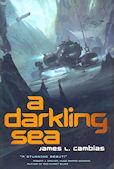
book review: A Darkling Sea

James L. Cambias.
A Darkling Sea.
Tor. 2014

---

Ilmatar is home to a newly-discovered alien species, that lives in total darkness under thick ice, at extremely high pressures and deadly cold, building a civilisation around the energy available from hot vents. Humans have a scientific base nearby, observing the aliens. But they are forbidden from interacting with them by the Sholen, another alien species that so nearly destroyed itself that it now insists on consensus in everything, and minimising any interference with new contacts. But then the meddling humans accidentally make contact with the Ilmatarans, which might lead to war with the not-so-unified Sholen.

This is an interesting view of three very different species: the relatively primitive Ilmatarans, the superior but reclusive Sholen, and the humans. None of these is a homogeneous culture: the plot is driven as much by conflicts within as between species. Not all the Sholens are that convinced of consensus and there are different political sub-groups to be considered; not all the Ilmatarans are civilised; not all the humans are very scientific. There's a semi-amusing thread running through, as the humans and Sholens keep incorrectly predicting how the others will react, based on completely incorrect stereotypes they have of each other.

The majority of the plot takes place in the dark cold ocean beneath a kilometer of ice, giving an extra claustrophobic edge to the tensions between the three species. The background is well drawn: the Ilmataran life-cycle, language and living arrangements are gradually revealed; how the humans can live below the ice is engagingly info-dumped. There are a couple of distressing deaths: these are not described in gory detail, leaving it to the imagination to fill in the blanks. Some of the humans seem to get much too worked up about events, while others seem surprisingly unemotional about everything. But on the whole, this is an interesting story about conflicts between species who have completely different philosophies that are partly a result of their completely different physiologies.

---

For all my book reviews, see my main website.

film review: Solo: A Star Wars Story

Where Rogue One was a prequel, showing how the situation at the start of the events of Star Wars – A New Hope arose, Solo is an origin story, showing how the character of Han Solo became who he was. We see how Han got the name “Solo”, how he met Chewbacca, how he won the Millennium Falcon from Lando Calrissian in a dodgy card game, how he made the Kessel Run in less than 12 parsecs (with a bit of hasty ret-conning why that even makes sense), and some things we didn’t know from previous films, such as how he joined the Imperial Army, the world and people he left behind, and how he was in at the genesis of the Rebellion.

no longer Solo

cocky kid

There is sufficient plot that this is an exciting stand-alone adventure of trust and betrayal, and also sufficient hooks to what comes later to make it a significant addition to the canon. My main gripe is that this is supposed to introduce us to the cynical Han Solo we know as an adult, by introducing him as a sort of "lovable rogue with a heart of gold"; but he’s just a bratty kid, really.

There is clearly meant to be a sequel, the “Jabba the Hut years”, maybe, since this ends well before episode IV kicks off, with a major part of the plot arc with his childhood sweetheart unresolved. We have to hope that the film does well enough not to end up with a prophetic title.

---

For all my film reviews, see my main website.

a student of the t-test

Statistics tests can seem like magic, but many of them work on the same underlying principle.  The starting point is usually some null hypothesis (which you hope to refute):

• you have some (possibly conceptual) population \(P\) of individuals, from which you can take a sample
• there is some statistic \(S\) of interest for your problem (the mean, the standard deviation, ...)
• you have a null hypothesis that your population \(P\) has the same value of the statistic as some reference population (for example, null hypothesis: the mean size of my treated population is the same as the mean size of the untreated population)

A statistical test of this hypothesis can work as follows:

• the statistic \(S\) will have as a corresponding sampling distribution \(X\)
• this is the distribution of the original statistic \(S\) if you measure it over many samples (for example, if you measure the mean of a sample, some samples will have a low mean – you were unlucky enough to pick all small members, sometimes a high mean – you just happened to pick all large members, but mostly a mean close to the true population mean)
• if you assume the population has some specific distribution (eg a normal distribution), you can often calculate this distribution \(X\)
• when you look at your actual experimental sample, you see where it lies within in this sampling distribution
• the sampling distribution \(X\) has some critical value, \(x_{crit}\), dependent on your desired significance \(\alpha\); only a small proportion of the distribution lies beyond \(x_{crit}\)
• your experimental sample has a value of the statistic \(S\), let’s call it \(x_{obs}\); if \(x_{obs} > x_{crit}\), it lies in that very small proportion of the distribution; this is deemed to be sufficiently unlikely to have happened by chance, and it is more likely that the null hypothesis doesn’t hold; so you reject the null hypothesis at the \(1-\alpha\) confidence level 

This is all a bit abstract, so let’s look in detail how it works for the Student’s \(t\)-test.  (This test was invented by the statistician William Sealy Gossett, who published under the pseudonym Student, hence the name.)  One of the nice things about having access to a programming language is that we can look at actual samples and distributions, to get a clearer intuition of what is going on.  I’ve used Python to draw all the charts below.

Let’s assume we have the following conceptual setup. We have a population of items, with a population mean \(\mu\) and population variance \(\sigma^2\). From this we draw a sample of n items. We calculate a statistic of that sample (for example, the sample mean \(\bar{x}\) or the sample variance \(s^2\)). We then draw another sample (either assuming we are drawing ‘with replacement’, or assuming that the population is large enough that this doesn’t matter), and calculate its relevant statistic. We do the \(r\) times, so we have \(r\) values of the statistic, giving us a distribution of that statistic, which we show in a histogram.  Here is the process for a population (of circles) with a uniform distribution of sizes (radius of the circles) between 0 and 300, and hence a mean size of 150.

Even with 3000 samples, that histogram looks a bit ragged.  Mathematically, the distribution we want is the one we get in the limit as the number of samples tends to infinity.  But here we are programming, so we want a number of samples that is ‘big enough’.

The chart below uses a population with a standard normal distribution (mean zero, standard deviation 1), and shows the sampling distribution that results from calculating the mean of the samples.  We can see that by the time we have 100,000 samples, the histogram is pretty smooth.

So in what follows, we use 100,000 samples in order to get a good view of the underlying distribution.  An the population will always be a normal distribution.

In the above example, there were 10 items per sample.  How does the size of the sample (that is, the number of items in each sample, not the number of different samples) affect the distribution?

The chart below takes 100,000 samples of different sizes (3, 5, 10, 20), and shows the sampling distributions of (top) the means and (middle) the standard deviations of those samples.  The bottom chart is a scatter plot of the (mean, sd) for each sample.

So we can see a clear effect on the size of samples drawn from the normal distribution

• for larger samples, the sample means are more closely distributed around the population mean (of 0) – larger samples give a better estimate of the underlying population mean
• for larger samples, the sample standard deviations are more closely and more symmetrically distributed around the population std dev (of 1) – larger samples give a better estimate of the underlying population s.d.

The distribution of means varies with the underlying distribution (its mean and standard deviation) as well as the size of samples taken. We can reduce this effect by calculating a different statistic, the \(t\)-statistic, rather than the sample mean \(\bar{x}\).
$$ t = \frac{\bar{x}-\mu}{s / \sqrt{n}}$$ The chart below shows how the distribution of the \(t\)-statistic varies with sample size.

In the limit that the number of samples tends to infinity, and where the underlying population has a normal distribution with a mean of \(\mu\), then this is the ‘\(t\)-distribution with \(n-1\) degrees of freedom’. Overlaying the plots above with the \(t\)-distribution shows a good fit.

The \(t\)-distribution does depend on the sample size, but not as extremely as the distribution of means:

Note that the underlying distribution being sampled is normal with a mean of \(\mu\), but the sd is not specified. To check whether this is important, the chart below shows the sampling distribution with a sample size of 10, from normal distributions with a variety of sds:

But what if we have the population mean wrong? That is, what if we assume that our samples are drawn from a population with a mean of \(\mu\) (the \(\mu\) used in the \(t\)-statistic), but it is actually drawn from a population with a different mean?  The chart below shows the experimental sampling distribution, compared to the theoretical \(t\)-distribution:

So, if the underlying distribution is normal with the assumed mean, we get a good match, and if it isn’t, we don’t. This is the basis of the \(t\)-test.

• First, define \(t_{crit}\) to be the value for \(t\) such that the area under the sampling distribution curve outside \(t_{crit}\) is \(\alpha\) (\(\alpha\) is typically 0.05, or 0.01).
• Calculate \(t_{obs}\) of your sample.  The probability of it falling outside \(t_{crit}\) if the null hypothesis holds is \(\alpha\), a small value.  The test says if this happens, it is more likely that the null hypothesis does not hold than you were unlucky, so reject the null hypothesis (with confidence \(1-\alpha\), 95% or 99% in the cases above).
• There are four cases, illustrated in the chart below for three different sample sizes:
• Your population has a normal distribution with mean \(\mu\)
• The \(t\)-statistic of your sample falls inside \(t_{crit}\) (with high probability \(1-\alpha\)).  You correctly fail to reject the null hypothesis: a true negative.
• The \(t\)-statistic of your sample falls outside \(t_{crit}\) (with low probability \(\alpha\)).  You incorrectly reject the null hypothesis: a false positive.
• Your population has a normal distribution, but with a mean different from \(\mu\)
• The \(t\)-statistic of your sample falls inside \(t_{crit}\). You incorrectly fail to reject the null hypothesis: a false negative.
• The \(t\)-statistic of your sample falls outside \(t_{crit}\).  You correctly reject the null hypothesis: a true positive.

Note that there is a large proportion of  false negatives (red areas in the chart above).  You may have only a small change of incorrectly rejecting the null hypothesis when it holds (high confidence), but may still have a large chance of incorrectly failing to reject it when it is false (low statistical power).  You can reduce this second error by increasing your sample size, as shown in the chart below (notice how the red area reduces as the sample size increases).

So that is the detail for the \(t\)-test assuming a normal distribution, but the same underlying philosophy holds for other tests and other distributions: a given observation is unlikely if the null hypothesis holds, assuming some properties of the sampling distribution (here that it is normal), so reject the null hypothesis with high confidence.

But what about the \(t\)-test if the sample is drawn from a non-normal distribution?  Well, it doesn’t work, because the calculation of \(t_{crit}\) is derived from the \(t\)-distribution, which assumes an underlying a normal population distribution.

sequestering carbon, several books at a time LXXXVII

The latest batch, mostly birthday presents:

overselling the weather

We haven’t had any rain for over seven weeks, and the garden is really suffering.  So we are constantly checking the forecast to see when this drought might end.  Here’s what my BBC Weather app says for next Wednesday:

Yay ! Rain at last!

So, we can look forward to the drought breaking on Wednesday, then?  Great!  When will it start to rain?  Let’s look at the hour-by-hour breakdown:

Umm

So, it’s going to rain for less than an hour?  How does that make the whole day summary be “light rain showers” and the background a dull grey?

And actually, there’s a mere 12% chance it will rain then.

Yet there’s a 17% chance of rain at 4pm, but no raindrop on that hour’s icon.

What do these symbols and percentages even mean?

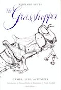
book review: The Grasshopper

Bernard Suits.
The Grasshopper: games, life, and utopia: 3rd edn.
Broadview Press. 2014

---

There are two main components to this book: (i) a definition of what constitutes a game; (ii) an argument that, since in Utopia, playing games is the only thing worth doing, that playing games is the supreme good. Suits spends some of the time building the framework needed for the definition of a game, but most of the time then arguing that the definition is correct, and about the overriding value of games.

First, the definition of a game, both long form, and snappy:

[p43] To play a game is to attempt to achieve a specific state of affairs [prelusory goal], using only means permitted by rules [lusory means], where the rules prohibit use of more efficient in favour of less efficient means [constitutive rules], and where the rules are accepted just because they make possible such activity [lusory attitude]. I also offer the following simpler and so to speak more portable version of the above: playing a game is the voluntary attempt to overcome unnecessary obstacles.

The long form is just a more precise framing of the snappy version, which is short, clear, and to the point: the voluntary attempt to overcome unnecessary obstacles. There are no wasted words. A game must be voluntary, not compulsory (so much for those compulsory “games” in school then); it is an attempt to overcome, success is not required, trying is sufficient; there must be an obstacle, so it isn’t some trivial activity, but requires some effort; and that obstacle must be unnecessary, for it it were necessary, overcoming it would be a job, or for survival, or some other reason.

This definition seems very reasonable, and gets around Wittgenstein’s claim that there is no sufficient and necessary conditions for something to be a game, by moving up a level of abstraction. Suits spends time picking apart his definition, and showing how various activities do, and do not, fit, and that those activities are, and are not, games, respectively.

So far, so good. Suits’ second argument is about the role of games in Utopia. In Suits’ Utopia there is no need to work; there is abundance of goods, companionship, and sexual partners for all; there is no physical or mental illness. That is, there is no need for involuntary activity, and there are no necessary obstacles to overcome. So the only worthwhile thing left to do in Utopia is play games:

[p188] I believe that Utopia is intelligible and I believe that game playing is what makes Utopia intelligible. What we have shown thus far is that there does not appear to be any thing to do in Utopia, precisely because in Utopia all instrumental activities have been eliminated. There is nothing to strive for precisely because everything has already been achieved. What we need, therefore, is some activity in which what is instrumental is inseparably combined with what is intrinsically valuable, and where the activity is not itself an instrument for some further end. Games meet this requirement perfectly.

I’m not convinced there is nothing to do in this Utopia other than play games. What about learning to play a musical instrument? That doesn’t seem to be a game: it is (in Utopia, at least) voluntary, but where is the unnecessary obstacle? One might argue that one could get a machine to play the music: is requiring the music be produced by oneself an unnecessary requirement? Listening and performing is qualitatively different, however.

But there is a deeper problem: I am not convinced that this Utopia can exist. Even if we assume perfect mental health, so no-one coerces anyone to do anything against their will (everything is voluntary), this does not imply there will be someone else to engage in any particular activity with you. Suits claims that

[p183] Under present conditions, there is a short supply of willing sexual objects relative to demand. And it may be surmised that the reason for this is the prevalence of inhibitions in the seekers of such objects, in the objects themselves, or in both, so that great expenditures of instrumental effort are required in order to overcome them and thus get at the intrinsic object of desire. But with everyone enjoying superb mental health the necessity for all this hard work is removed and sexual partners are every bit as accessible as yachts and diamonds.

This totally misses the point: sexual partners (or even tennis partners) are not “objects” in anything like the same sense that yachts and diamonds are objects. They are people, with their own desires, which, even with their posited perfect mental health, need not overlap with yours.

But let us for the sake of argument agree that if such a Utopia were to exist, then the only worthwhile thing to do there is play games. Suits goes further, and has his narrator (the eponymous Grasshopper) make an extraordinary claim: that because games have this status of being the only worthwhile thing to do in Utopia, that they are the only worthwhile thing for him to do in this world; he will only play games, will do no work, and so will starve to death come winter. He won’t even do a little work in order to live longer and thereby play more games: doing so would be the death of his essence as the Grasshopper (although he seems quite willing to lecture his acolytes rather than play). This seems a little fanatical. However, he does say to his acolytes that:

[p9] I agree that the principles in question are worth dying for. But I must remind you that they are the principles of Grasshoppers. I am not here to persuade you to die for my principles, but to persuade you that I must.

Oh that all fanatical believers took such a view of their beliefs! But in a sense, this reinforces my view of Utopia: what if, instead of dying for his principles, the Grasshopper wanted to play a new game:

I agree that the game in question is worth playing. But I must remind you that this is a game of Grasshoppers. I am not here to persuade you to play my game, but to persuade you that I must.

But what if the game requires other players, and there are no other players wishing to play? One cannot require that Utopia be populated with other players for one’s own benefit. Robot players may not be sufficient: playing against another person may be an unnecessary obstacle, but if that’s part of the game…

I found this a fascinating and thought-provoking book. The definition of a game is excellent: compact enough to be memorable; simple enough to be applicable; abstract enough to show the virtue of abstraction. The consequences of the definition are not so apparent to me, but it is an interesting journey to follow the argument: in my Utopia, reading such books would be more worthwhile that playing games.

---

For all my book reviews, see my main website.

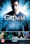
TV review: Grimm season 6

!!! SPOILERS FOR SEASON 5 !!!
.
.
.
.
.

This sixth and final (half) season starts where season 5 ended: Black Claw leader Bonaparte dead by Reynard’s Diana-controlled hand. This leads into a frantic set of episodes, where monster-of-the-week vies with a scramble to tie up all the loose ends in only 13 episodes. Black Claw conveniently disappears in a puff of smoke, while the arc focusses on the Magic Stick and what it means, leading up to a potential catastrophe that could destroy the entire human world. (Well, if you are going to potentially save the world, best to leave it to the end, otherwise it’s hard to top.)

There were possibilities for “happy” endings that would have been annoying resets: these possibilities were not taken. However, there were hanging guns that never went off (Black Claw conveniently vanishing; Diana conveniently not destroying the world in a fit of pique; re-hexenbiested-Adelinde conveniently not reverting to a monster). Also note: if you kill one major character, viewers might think they are really dead even in a fantasy series. When you kill them all, viewers are more suspicious. Despite these issues, the season did tie up most loose ends, without giving the impression that the characters’ adventures over.

---

For all my SF TV reviews, see my main website.

book review: Meddling Kids

Edgar Cantero.
Meddling Kids.
Titan Books. 2018

---

Scooby-Doo meets The Famous Five meets Cthulhu.

As teens, the Blyton Summer Detective Club had adventures tracking down puzzles and unmasking the bad guys. Their final case was discovering who was behind the Sleepy Lake Monster. Since then, they’ve grown up, and grown apart, and fallen apart: one in jail; one an alcoholic drinking away the nightmares; one in an asylum; one dead. Did they really solve their last case, or was there more to it, that has caused their individual problems? The gang reassembles (yes, even the dead member) to put the past to rest permanently.

This could have been played purely for laughs, but, although there are some humorous moments, chasing down eldritch lake monsters is a serious business, with serious consequences. The serious parts, and the parts subverting various tropes, work much better than the attempts at (slapstick) humour, so it’s just as well they are in the majority.

The presence of the gang’s ghostly leader (even though he might be only in Nate’s head?), plus the current traumatised state of the gang, suggests early on that this isn’t going to be resolved by ripping off yet another costume from yet another con artist. So the main things to puzzle out are the identity of the bad guy, and how to save the world from total annihilation.

This starts off a bit slow, with the gang reassembling, but then crackles along. I enjoyed the trope subversion, in particular the way certain stock characters from the gang’s past had also grown up and changed. And also the way some at-the-time implausibilities are later shown to be plot-relevant. A fun reimagining.

---

For all my book reviews, see my main website.

sequestering carbon, several books at a time LXXXVI

The latest batch, including proceedings from the recent UCNC conference:

bouncing around Europe?

I’d left Durham on the 16:48 train to York, and about 20 minutes into my journey I thought I’d track progress using my phone GPS.  There was no 4G signal out in deepest Northern England, but the GPS usually plots its position on Google Maps nevertheless.

hmm.  I appear to be in Paris?!

Some glitch, presumably.  A couple of minutes later I seemed to have returned north.

that’s more like it!

But not much later than that, I appeared to be back in Paris.

And then two minutes later, north again:

After that, it sort of gave up the ghost until I got close to York, when it gave me a position in a huge blue circle of uncertainty.  Was the train interfering with the GPS signal?  It doesn’t usually; this is a game I often play on the train, and the first time I’ve seen this happen.

What’s weird about the Paris location is that, although I was in Paris a week ago, catching the Eurostar home, I was nowhere near the Paris location shown by the GPS.

If Google is logging my GPS position (like it does), then it should be getting mighty confused about my travels!

Isn’t technology wonderful?