We can see clearly now the spider webs are gone.
Friday, 29 May 2020
Covid-19 diary: seeing clearly
Labels:
Covid-19
The window cleaners came today for the first time since lockdown.
Thursday, 28 May 2020
Wednesday, 27 May 2020
Covid-19 diary: eye tests
Dominic Cummings has said that he drove to Barnard Castle with his wife and child at the end of his lockdown-busting trip to County Durham in order to test his eyesight before making the long drive home to London.
If the Indepedent’s report is accurate (and I have no reason to believe otherwise; there is plenty of other evidence), then here are only two possibilities:
- Cummings is lying about his reason for his actions
- Cummings is telling the truth about his reasons for his actions
If he is lying, then he should be sacked for this lie.
If he is telling the truth, then he should be sacked for being too stupid to be a government advisor.
Additionally, if he is telling the truth, and he is happy to risk his wife and child’s life in such a manner, then it rather calls into question his original excuse for travelling north: worry for his child’s well being.
Sunday, 24 May 2020
rational conics
Labels:
books,
geometry,
mathematics,
python
I’m currently reading Elliptic Tales, some light relief from lockdown. On reading the preface alone, I discovered something I hadn’t known before. This might be quite well-know to people with a “traditonal” maths background, but I did “modern maths” at school: lots of cool set and group theory, very little classical geometry.
The discussion in the book is just about circles, but a little googling helped me discover this is a result that applies more broadly.
Consider the general quadratic equation of two variables:
\(a x^2 + b x y + c y^2 + d x + e y + f = 0\)
where not all of the coefficients of the quadratic terms, \(a,b,c\), are zero. Depending on the coefficent values, this gives a circle, ellipse, parabola, or hyperbola, that is, a conic section.
Let’s now consider the restricted case where all the coefficients are rational numbers. A rational solution to this equation is a solution \((x,y)\) where both \(x\) and \(y\) are rational numbers.
Now comes the interesting bit. Take a straight line with rational slope, \(y = q x + r\), where \(q\) is rational, that cuts the quadratic curve at two points. Then either both points are rational solutions, or neither is.
The book proves this for the case of a circle, and then shows how to use the result to find all the rational points on the unit circle, \(x^2+y^2=1\). You need one point that you know is rational, so let’s chose \((-1,0)\). Then draw a straight line with rational slope that crosses the \(y\) axis at \(q\); that is, \(q\) is rational. This line has equation \(y=q(x+1)\). Then solve for the other point where the line crosses the circle to get a rational solution:
It is clear from the form of the solution that if \(q\) is rational, so is the point \((x_q,y_q)\). Additionally, there are no rational solutions that correspond to an irrational value of \(q\), so we can use \(q\) to parameterise all the rational solutions.
Notice also that if we scale up the yellow right-angled triangle, multiplying it by a suitable integer \(n\), so that both \(n x_q\) and \(n y_q\) are integers, the three sides form a Pythagorean triple.
These points and triples can be generated very easily, just by scanning through values of \(q\) and printing out the unique triples. And Python’s fraction module makes this particularly straightforward (with a bit of fiddling to print in a fixed width format to make things line up neatly; yes, I’m a bit picky about things like this):
So I’ve only read the Preface so far, and yet I’ve already learned some interesting stuff, and had an excuse to play with Python. Let’s hope the rest is as good (but I suspect it will rapidly get harder…)
The discussion in the book is just about circles, but a little googling helped me discover this is a result that applies more broadly.
Consider the general quadratic equation of two variables:
\(a x^2 + b x y + c y^2 + d x + e y + f = 0\)
where not all of the coefficients of the quadratic terms, \(a,b,c\), are zero. Depending on the coefficent values, this gives a circle, ellipse, parabola, or hyperbola, that is, a conic section.
Let’s now consider the restricted case where all the coefficients are rational numbers. A rational solution to this equation is a solution \((x,y)\) where both \(x\) and \(y\) are rational numbers.
Now comes the interesting bit. Take a straight line with rational slope, \(y = q x + r\), where \(q\) is rational, that cuts the quadratic curve at two points. Then either both points are rational solutions, or neither is.
The book proves this for the case of a circle, and then shows how to use the result to find all the rational points on the unit circle, \(x^2+y^2=1\). You need one point that you know is rational, so let’s chose \((-1,0)\). Then draw a straight line with rational slope that crosses the \(y\) axis at \(q\); that is, \(q\) is rational. This line has equation \(y=q(x+1)\). Then solve for the other point where the line crosses the circle to get a rational solution:
It is clear from the form of the solution that if \(q\) is rational, so is the point \((x_q,y_q)\). Additionally, there are no rational solutions that correspond to an irrational value of \(q\), so we can use \(q\) to parameterise all the rational solutions.
Notice also that if we scale up the yellow right-angled triangle, multiplying it by a suitable integer \(n\), so that both \(n x_q\) and \(n y_q\) are integers, the three sides form a Pythagorean triple.
These points and triples can be generated very easily, just by scanning through values of \(q\) and printing out the unique triples. And Python’s fraction module makes this particularly straightforward (with a bit of fiddling to print in a fixed width format to make things line up neatly; yes, I’m a bit picky about things like this):
from fractions import Fraction as frac

found = set()
for denom in range(1,15):
    for num in range(1,denom):
        q = frac(num,denom)
        xq = (1-q*q)/(1+q*q)
        yq = 2*q/(1+q*q)

        n = xq.denominator
        triple = sorted([int(xq*n), int(yq*n), n])

        if triple[0] not in found:
            print( '{0:<7}  ({1:^7}, {2:^7})  {3}'.format(str(q),str(xq),str(yq),triple) )
            found.add(triple[0])
1/2      (  3/5  ,   4/5  )  [3, 4, 5]
2/3      ( 5/13  ,  12/13 )  [5, 12, 13]
1/4      ( 15/17 ,  8/17  )  [8, 15, 17]
3/4      ( 7/25  ,  24/25 )  [7, 24, 25]
2/5      ( 21/29 ,  20/29 )  [20, 21, 29]
4/5      ( 9/41  ,  40/41 )  [9, 40, 41]
1/6      ( 35/37 ,  12/37 )  [12, 35, 37]
5/6      ( 11/61 ,  60/61 )  [11, 60, 61]
2/7      ( 45/53 ,  28/53 )  [28, 45, 53]
4/7      ( 33/65 ,  56/65 )  [33, 56, 65]
6/7      ( 13/85 ,  84/85 )  [13, 84, 85]
1/8      ( 63/65 ,  16/65 )  [16, 63, 65]
3/8      ( 55/73 ,  48/73 )  [48, 55, 73]
5/8      ( 39/89 ,  80/89 )  [39, 80, 89]
7/8      (15/113 , 112/113)  [15, 112, 113]
2/9      ( 77/85 ,  36/85 )  [36, 77, 85]
4/9      ( 65/97 ,  72/97 )  [65, 72, 97]
8/9      (17/145 , 144/145)  [17, 144, 145]
3/10     (91/109 , 60/109 )  [60, 91, 109]
7/10     (51/149 , 140/149)  [51, 140, 149]
9/10     (19/181 , 180/181)  [19, 180, 181]
2/11     (117/125, 44/125 )  [44, 117, 125]
4/11     (105/137, 88/137 )  [88, 105, 137]
6/11     (85/157 , 132/157)  [85, 132, 157]
8/11     (57/185 , 176/185)  [57, 176, 185]
10/11    (21/221 , 220/221)  [21, 220, 221]
1/12     (143/145, 24/145 )  [24, 143, 145]
5/12     (119/169, 120/169)  [119, 120, 169]
7/12     (95/193 , 168/193)  [95, 168, 193]
11/12    (23/265 , 264/265)  [23, 264, 265]
2/13     (165/173, 52/173 )  [52, 165, 173]
4/13     (153/185, 104/185)  [104, 153, 185]
6/13     (133/205, 156/205)  [133, 156, 205]
8/13     (105/233, 208/233)  [105, 208, 233]
10/13    (69/269 , 260/269)  [69, 260, 269]
12/13    (25/313 , 312/313)  [25, 312, 313]
3/14     (187/205, 84/205 )  [84, 187, 205]
5/14     (171/221, 140/221)  [140, 171, 221]
9/14     (115/277, 252/277)  [115, 252, 277]
11/14    (75/317 , 308/317)  [75, 308, 317]
13/14    (27/365 , 364/365)  [27, 364, 365]
and larger values are readily calculated, such as:
500/1001 (752001/1252001, 1001000/1252001) [752001, 1001000, 1252001]
So I’ve only read the Preface so far, and yet I’ve already learned some interesting stuff, and had an excuse to play with Python. Let’s hope the rest is as good (but I suspect it will rapidly get harder…)
Saturday, 23 May 2020
Sunday, 17 May 2020
the Buddhabrot
Labels:
fractals,
mathematics,
python
As we have seen, the Mandelbrot set can be calulated by iterating a function, and testing whether the sequence it generates diverges or not. The so-called Buddhabrot (named for its appearance) looks at the trajectory of the generated sequence, as the generated points hop about, diverging or not. Points that start with a \(c\) value outside the Mandelbrot set, and so produce diverging sequences, may nevertheless have points along the way that land inside the set.
The Buddhabrot takes all the points ourside the set, and plots each point in the trajectory to divergence. This leads to a density map: some points are visited more often than others (it is conventional to plot this rotated 90 degrees, to highlight the shape):
In addition, there is the anti-Buddhabrot, which plots the trajectories of all the \(c\) values inside the Mandelbrot set. These do not diverge: some converge inside the set, others cycle around.
Again, the code is relatively simple, and you can calculate the Buddhabrot and anti-Buddhabrot at the same time:
As before, we can iterate using different powers of \(k\), and get analogues of the Buddhabrot.
More figures and animations of the Mandelbrot set, the Julia set, and the Buddhabrot, are available on my website.
The Buddhabrot takes all the points ourside the set, and plots each point in the trajectory to divergence. This leads to a density map: some points are visited more often than others (it is conventional to plot this rotated 90 degrees, to highlight the shape):
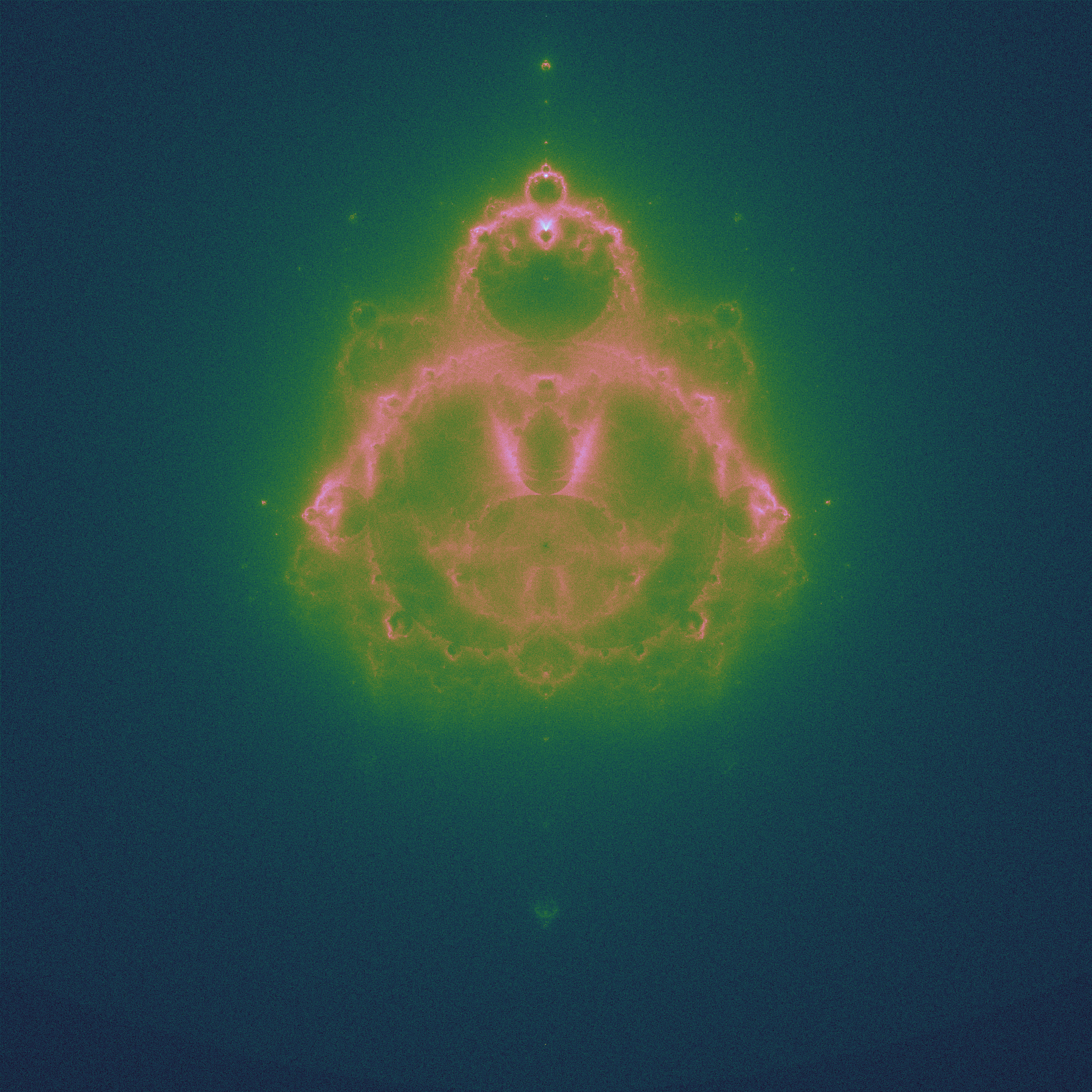 |
| 42 million randomly chosen values of \(c\) |
Again, the code is relatively simple, and you can calculate the Buddhabrot and anti-Buddhabrot at the same time:
import numpy  as np
import matplotlib.pyplot as plt

IMSIZE = 2048 # image width/height
ITER = 1000

def mandelbrot(c, k=2):
    # c = position, complex; k = power, real
    z = c
    traj = [c]
    for i in range(1, ITER):
        z = z ** k + c
        traj += [z]
        if abs(z) > 2: # escapes
            return traj, []
    return [], traj

def updateimage(img, traj):
    for z in traj:
        xt, yt = z.real, z.imag
        ixt, iyt = int((2+xt)*IMSIZE/4), int((2-yt)*IMSIZE/4)
        # check traj still in plot area
if 0 <= ixt and ixt < IMSIZE and 0 <= iyt and iyt < IMSIZE:
            img[ixt,iyt] += 1

# start with value 1 because take logs later
buddha = np.ones([IMSIZE,IMSIZE])
abuddha = np.ones([IMSIZE,IMSIZE])
for i in range(IMSIZE*IMSIZE*10):
    z = np.complex(np.random.uniform()*4-2, np.random.uniform()*4-2)
    traj, traja = mandelbrot(z, k)
    updateimage(buddha,traj)
    updateimage(abuddha,traja)

buddha = np.square(np.log(buddha)) # to extend small numbers
abuddha = np.log(abuddha)          # to extend small numbers

plt.axis('off')
plt.imshow(buddha, cmap='cubehelix')
plt.show()
plt.imshow(abuddha, cmap='cubehelix')
plt.show()
These plots are more are computationally expensive to produce than the plain Mandelbrot set plots: it is good to have a large number of initial points, and a long trajectory run. There are some beautifully detailed figures on the Wikipedia page.As before, we can iterate using different powers of \(k\), and get analogues of the Buddhabrot.
 |
| \(k = 2.5\), the "piggy-brot" |
Saturday, 16 May 2020
Julia set
Labels:
fractals,
mathematics,
python
Before the Mandelbrot set came the closely related Julia set.
Consider the sequence \(z_0=z; z_{n+1} = z_n^2 + c\), where \(z\) and \(c\) are complex numbers. Consider a given value of \(c\). Then for some values of \(z\), the sequence diverges to infinity; for other values it stays bounded. The Julia set is the border of the region(s) between which the values of \(z\) do or do not diverge. Plotting these \(z\) points in the complex plane (again plotting the points that do diverge in colours that represent how fast they diverge) gives a picture that depends on the value of \(c\):
If the point \(c\) is inside the Mandelbrot set, the corresponding Julia set is one connected border around one connected region. If it is outside, there are instead many disconneted regions. The deeper inside the Mandelbrot set, the larger and rounder the black region in the Julia set looks; the further outside the Mandelbrot set, the smaller and hence paler he Julia set looks.
This leads to the idea of plotting the Mandelbrot set in a rather different way. For each value of \(c\), instead of plotting a pixel in a colur representing the speed of divergence, plot a little image of the associated Julia set, whose overall colour is related to the speed of divergence:
As with the Mandelbrot set, we can construct related fractals by iterating different powers, \(z_0=z; z_{n+1} = z_n^k + c\):
The code is just as simple as, and very similar to, the Mandelbrot code, too:
Consider the sequence \(z_0=z; z_{n+1} = z_n^2 + c\), where \(z\) and \(c\) are complex numbers. Consider a given value of \(c\). Then for some values of \(z\), the sequence diverges to infinity; for other values it stays bounded. The Julia set is the border of the region(s) between which the values of \(z\) do or do not diverge. Plotting these \(z\) points in the complex plane (again plotting the points that do diverge in colours that represent how fast they diverge) gives a picture that depends on the value of \(c\):
 |
| \(c = -0.5+0.5i\), a point well inside the Mandelbrot set |
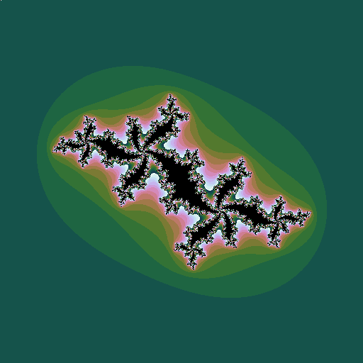 |
| \(c = -0.5+0.6i\), a point just inside the Mandelbrot set |
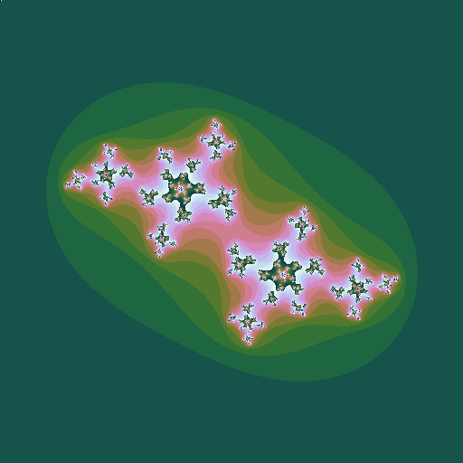 |
| \(c = -0.5+0.7i\), a point outside the Mandelbrot set |
This leads to the idea of plotting the Mandelbrot set in a rather different way. For each value of \(c\), instead of plotting a pixel in a colur representing the speed of divergence, plot a little image of the associated Julia set, whose overall colour is related to the speed of divergence:
 |
| Julia sets mapping out the Mandelbrot set |
As with the Mandelbrot set, we can construct related fractals by iterating different powers, \(z_0=z; z_{n+1} = z_n^k + c\):
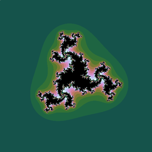 |
| \(k=3, c = -0.5+0.598i\) |
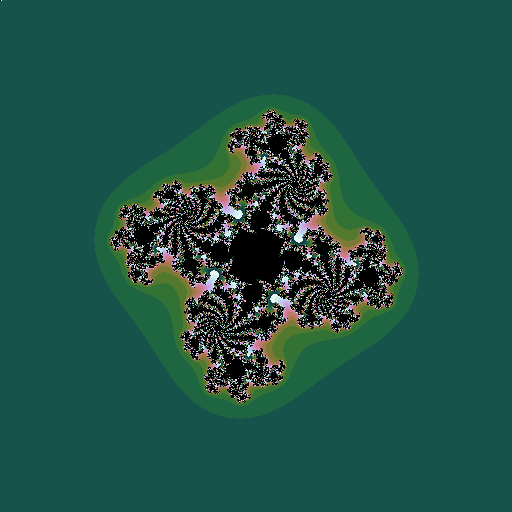 |
| \(k=4, c = -0.5+0.444i\) |
The code is just as simple as, and very similar to, the Mandelbrot code, too:
import numpy  as np
import matplotlib.pyplot as plt

IMSIZE = 512 # image width/height
ITER = 256

def julia(z, c, k=2):
    # z = position, complex ; c = constant, complex; k = power, real
    z = z
    for i in range(1, ITER):
        z = z ** k + c
        if abs(z) > 2:
            return 4 + i % 16 #16 colours
    return 0

julie = np.zeros([IMSIZE,IMSIZE])
c = np.complex(-0.5,0.5)

for ix in range(IMSIZE):
    x = 4 * ix / IMSIZE - 2
    for iy in range(IMSIZE):
        y = 2 - 4 * iy / IMSIZE
        julie[iy,ix] = julia(np.complex(x,y), c, 5)

julie[0,0]=0   # kludge to get uniform colour maps for all plots

plt.axis('off')
plt.imshow(julie, cmap='cubehelix')
plt.show()
Thursday, 14 May 2020
Mandelbrot set
Labels:
fractals,
mathematics,
python
When I reviewed Matt Pearson's Generative Art, and plotted a Mandelbrot set made from random splodges, I went and looked at my own webpage about this structure. I discovered a case of bit rot: the little Java applet I'd written many years ago had stopped working, as is the way with much old software. Rather than rewrite it, I pottered around in Python, reproducing some of the plots.
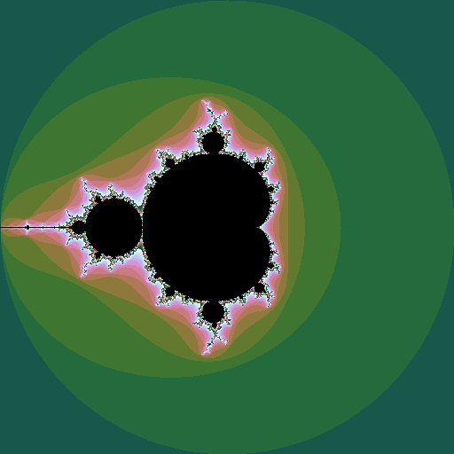
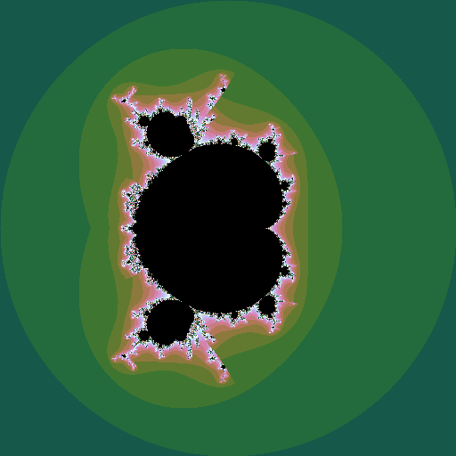
The Mandelborot set is a highly complex fractal generated from a very simple equation. Consider the sequence \(z_0=0; z_{n+1} = z_n^2 + c\), where \(z\) and \(c\) are complex numbers. For some values of \(c\), the sequence diverges to infinity; for other values it stays bounded. The Mandelbrot set is all the values of \(c\) for which the sequence does not diverge. Plotting these points in the complex plane (and plotting the points that do diverge in colours that represent how fast they diverge) gives the now well-known picture:
If \(z\) is raised to a different power, different sets are seen, still with complex shapes.
The power doesn't even need to be an integer.
The discontinuities visible are due to the fractional power resulting in a logarithm in the solutoin, which is multi-values in the complex plane. The plot shows only the principal value.
We can make an animation of the shape of the set as this power \(k\) changes:
One thing I love about the Mandelbrot set is the sheer simplicity of the code needed to plot it:
The Mandelborot set is a highly complex fractal generated from a very simple equation. Consider the sequence \(z_0=0; z_{n+1} = z_n^2 + c\), where \(z\) and \(c\) are complex numbers. For some values of \(c\), the sequence diverges to infinity; for other values it stays bounded. The Mandelbrot set is all the values of \(c\) for which the sequence does not diverge. Plotting these points in the complex plane (and plotting the points that do diverge in colours that represent how fast they diverge) gives the now well-known picture:
If \(z\) is raised to a different power, different sets are seen, still with complex shapes.
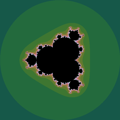 |
| iterating \(z^4 + c\) |
 |
| iterating \(z^{2.5} + c\) |
We can make an animation of the shape of the set as this power \(k\) changes:
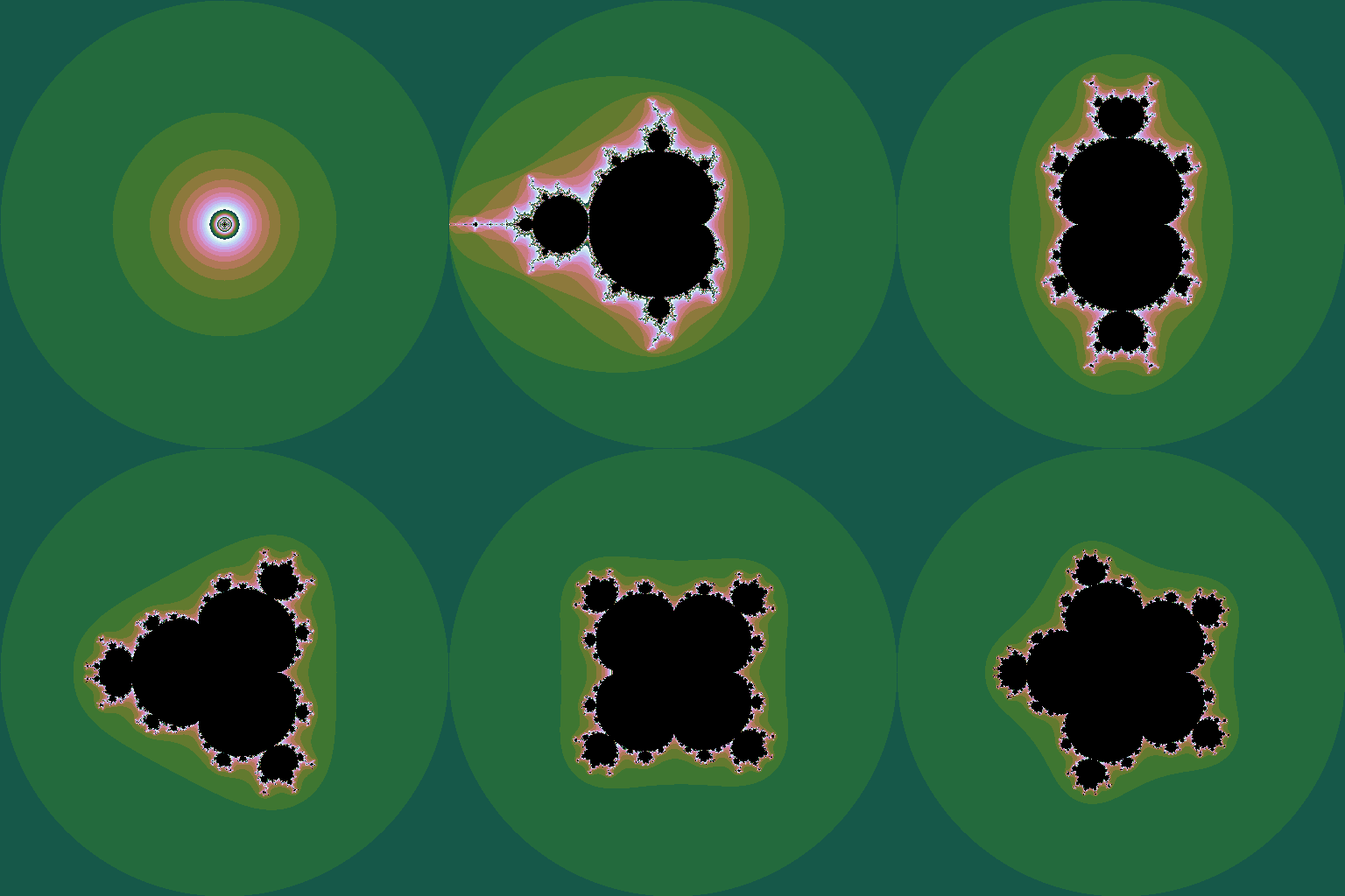 |
| \(k = 1 .. 6\), step \(0.05\) |
One thing I love about the Mandelbrot set is the sheer simplicity of the code needed to plot it:
import numpy  as np
import matplotlib.pyplot as plt

IMSIZE = 512 # image width/height
ITER = 256

def mandelbrot(c, k=2):
    # c = position, complex; # k = power, real
    z = c
    for i in range(1, ITER):
        if abs(z) > 2:
            return 4 + i % 16 #16 colours
        z = z ** k + c
    return 0

mandy = np.zeros([IMSIZE,IMSIZE])
for ix in range(IMSIZE):
    x = 4 * ix / IMSIZE - 2
    for iy in range(IMSIZE):
        y = 2 - 4 * iy / IMSIZE
        mandy[iy,ix] = mandelbrot(np.complex(x,y), k)

    plt.axis('off')
    plt.imshow(mandy, cmap='cubehelix')
    plt.show()
And there's more. But that's for another post.Friday, 8 May 2020
Covid-19 diary: VE day
Today we celebrate the 75th anniversary of the liberation of Europe from a brutal fascist dictatorship, and acknowledge the sacrifices our parents and grandparents made during the time.
The rise of the Nazis is an important lesson of history. It didn’t happen overnight; it was a gradual process. Not everyone subscribed to the ideology, but as its grip strengthened, it became increasingly difficult, and dangerous, to resist.
The lesson is that we should watch out for similar processes happening today, and nip them in the bud. There are currently distressing parallels of the rise of nationalism and fascism around the world, from nationalistic groups arising in European and other countries, including the nationalistic underpinnings of Brexit, to the nibbling away of the rule of law, of checks and balances, in other countries.
Crises can tend to amplify nationalism, as people pull together locally, but apart globally. And necessary measures put in place during crises can be difficult to remove after the crisis has passed (is it really over? better be safe than sorry!)
VE day reminds us of the utter horrors of fascism.
Don’t let Covid-19 help them return through the back door.
Tuesday, 5 May 2020
Covid-19 diary : snooker
The 2020 World Snooker Championship should have been on TV last week, but unsurprisingly it has been postponed. So BBC2 have been showing highlights of old matches. Ask anyone who has been around a few years which match they would definitely show, and you will get the answer “the 1985 final”. That final, between Steve Davies and Dennis Taylor, is the stuff of legend.
It was the best of 35 frames. It looked as if it was going to be over quickly, as Steve Davies took the first 8 frames. But then Taylor started coming back, and the match went into its second day. We decided to watch the end game, thinking Davies would probably clean up quite quickly. But then it reached 17 all.
The final frame was agonising, but riveting. It took over an hour, and went on past midnight. It was eventually decided on the black ball, which didn’t go down without a fight. Truly memorable, and there were a lot of bleary-eyed people at work the next day!
BBC2 showed it again at the end of last week. I watched the final frame. Again. I had forgotten the details of the agonising safety play, the foul strokes, the snookers, the missed pots, the green that ended up in a different pocket from where it was aimed. I held my breath during several shots. And then there was that final black, hanging on, with another succession of safety shots and missed pots. Eventually, Steve Davis missed a pot, and the white hit the black on the rebound, leaving a clear shot for Taylor; the look Davies gave the table when he saw what had happened.
In the interview afterward the repeat, we learned that nearly 19m people, nearly one third of the UK population, watched that final frame, after midnight, on BBC2. And we learned how snooker had grown; only 13 years earlier, in 1972, Hurricane Higgins won the championship playing in a cramped workingman’s club. David Attenborough was responsible for this growth, wanting a relatively cheap programme to show off the new colour television service.
One intersting little fact I got from Wikipedia: Taylor had not been in the lead at any point during the game, until he potted that final black to win the championship.
And I suppose that, if not for Covid-19, we might not have seen it again. It’s a funny old world.
Saturday, 2 May 2020
book review: Generative Design
Labels:
books,
graphics,
processing,
python,
review
Hartmut Bohnacker, Benedict Gross, Julia Laub, Claudius Lazzeroni.
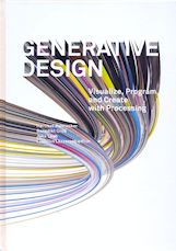
Generative Design: visualize, program, and create with Processing.
Princeton Architectural Press. 2012
Having read Pearson’s introduction to Generative Art with Processing I was in the mood to move on to the next level. Hence this book, also based on the interactive Processing language, but with many more, and more sophisticated, projects. These cover bothart and design.
The book is in three main parts. First, Project Selection, is over 100 pages of glossy pictures, whetting the appetite for what is to come. Second, we get Basic Principles, starting with an introduction to Processing, and chapters on working with colour, shape, text and images; these projects are quite sophisticated in their own right, but each focusses on a single aspect. Finally, we get Complex Methods: more ambitious projects combining the concepts introduced earlier.
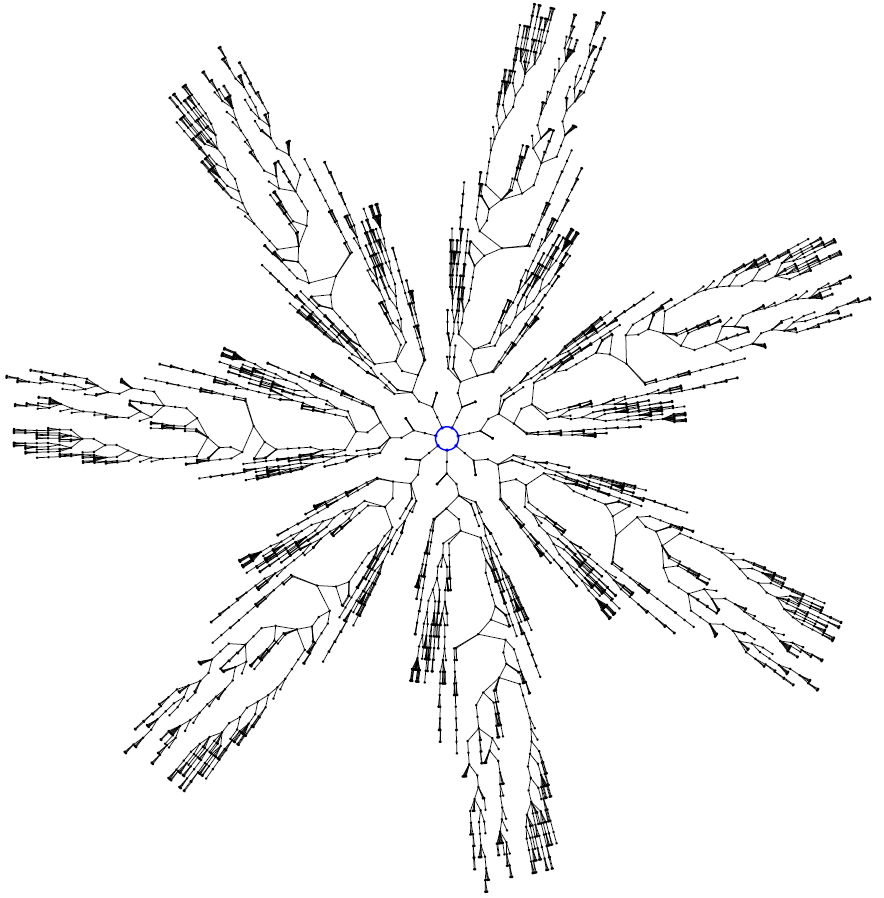
All the code is available online (in Java mode), which provides an incredibly rich resource to start working from. I didn’t directly use any of this code; I did, however, get inspiration from the Sunburst Trees project to write some of my own (Python) code to draw basins of attraction of elementary cellular automata:
A lovely book all round: great content, and beautifully typeset.
For all my book reviews, see my main website.
Generative Design: visualize, program, and create with Processing.
Princeton Architectural Press. 2012
Having read Pearson’s introduction to Generative Art with Processing I was in the mood to move on to the next level. Hence this book, also based on the interactive Processing language, but with many more, and more sophisticated, projects. These cover bothart and design.
The book is in three main parts. First, Project Selection, is over 100 pages of glossy pictures, whetting the appetite for what is to come. Second, we get Basic Principles, starting with an introduction to Processing, and chapters on working with colour, shape, text and images; these projects are quite sophisticated in their own right, but each focusses on a single aspect. Finally, we get Complex Methods: more ambitious projects combining the concepts introduced earlier.
All the code is available online (in Java mode), which provides an incredibly rich resource to start working from. I didn’t directly use any of this code; I did, however, get inspiration from the Sunburst Trees project to write some of my own (Python) code to draw basins of attraction of elementary cellular automata:

A lovely book all round: great content, and beautifully typeset.
For all my book reviews, see my main website.
Subscribe to:
Comments (Atom)


