Julia set

Before the Mandelbrot set came the closely related Julia set.

Consider the sequence \(z_0=z; z_{n+1} = z_n^2 + c\), where \(z\) and \(c\) are complex numbers.  Consider a given value of \(c\).  Then for some values of \(z\), the sequence diverges to infinity; for other values it stays bounded.  The Julia set is the border of the region(s) between which the values of \(z\) do or do not diverge.  Plotting these \(z\) points in the complex plane (again plotting the points that do diverge in colours that represent how fast they diverge) gives a picture that depends on the value of \(c\):

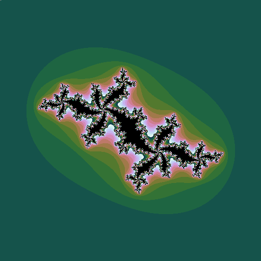
\(c = -0.5+0.5i\), a point well inside the Mandelbrot set

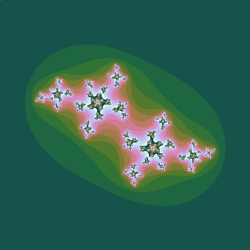
\(c = -0.5+0.6i\), a point just inside the Mandelbrot set

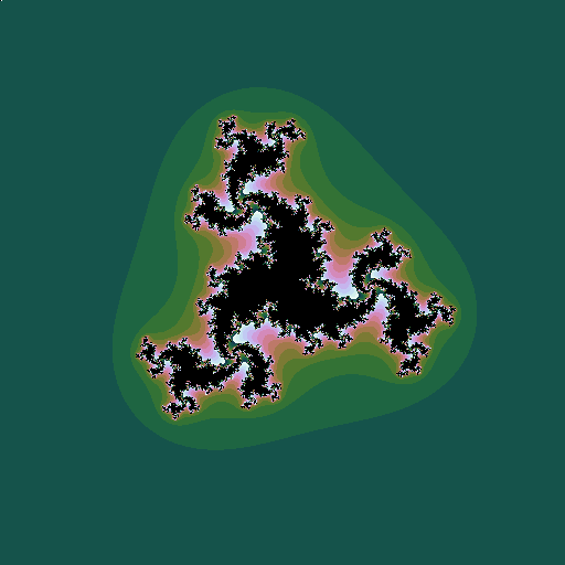
\(c = -0.5+0.7i\), a point outside the Mandelbrot set

If the point \(c\) is inside the Mandelbrot set, the corresponding Julia set is one connected border around one connected region.  If it is outside, there are instead many disconneted regions.  The deeper inside the Mandelbrot set, the larger and rounder the black region in the Julia set looks; the further outside the Mandelbrot set, the smaller and hence paler he Julia set looks.

This leads to the idea of plotting the Mandelbrot set in a rather different way.  For each value of \(c\), instead of plotting a pixel in a colur representing the speed of divergence, plot a little image of the associated Julia set, whose overall colour is related to the speed of divergence:

Julia sets mapping out the Mandelbrot set

As with the Mandelbrot set, we can construct related fractals by iterating different powers, \(z_0=z; z_{n+1} = z_n^k + c\):

\(k=3, c = -0.5+0.598i\)

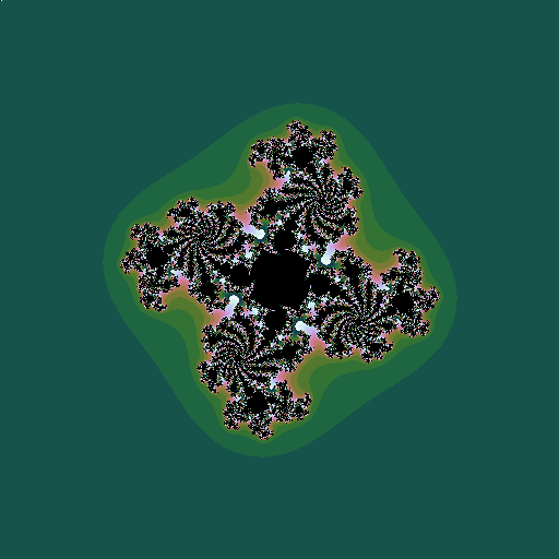\(k=4, c = -0.5+0.444i\)

The code is just as simple as, and very similar to, the Mandelbrot code, too:

import numpy  as np
import matplotlib.pyplot as plt

IMSIZE = 512 # image width/height 
ITER = 256

def julia(z, c, k=2): 
    # z = position, complex ; c = constant, complex; k = power, real
    z = z
    for i in range(1, ITER): 
        z = z ** k + c 
        if abs(z) > 2: 
            return 4 + i % 16 #16 colours
    return 0
    
julie = np.zeros([IMSIZE,IMSIZE]) 
c = np.complex(-0.5,0.5)

for ix in range(IMSIZE):  
    x = 4 * ix / IMSIZE - 2
    for iy in range(IMSIZE):
        y = 2 - 4 * iy / IMSIZE
        julie[iy,ix] = julia(np.complex(x,y), c, 5)
        
julie[0,0]=0   # kludge to get uniform colour maps for all plots

plt.axis('off')
plt.imshow(julie, cmap='cubehelix')
plt.show()